Overview
This chapter introduces Chemical Bonding and Molecular Structure — the foundation for understanding how atoms combine to form molecules and how molecular structure determines physical and chemical properties. Beginning with Lewis structures and the octet rule (including its exceptions), the chapter develops concepts of ionic and covalent bonding, coordinate (dative) bonds, and covalent character in ionic compounds. It presents classical and modern models that explain bond formation and molecular shape: Valence Bond Theory and hybridisation, VSEPR theory for predicting shapes and bond angles, and an introduction to Molecular Orbital Theory for diatomic molecules. Important allied ideas such as bond length, bond energy, bond order, polarity, dipole moment, resonance, formal charge, electronegativity, and Fajan’s rules are explained and applied to common molecules and ions. Importance: Understanding bonding and molecular structure is critical for predicting and rationalising reactivity, stability, physical properties (melting/boiling points, solubility, conductivity), magnetic behavior and spectroscopic features of substances. These concepts are central to inorganic, organic and…
Learning Objectives
- Define ionic, covalent and coordinate (dative) bonds and explain the basic mechanism of their formation
- Explain factors affecting ionic bond strength, lattice energy and typical physical properties of ionic compounds
- Construct Lewis structures for molecules and polyatomic ions, assign formal charges and identify resonance forms
- Apply VSEPR theory to predict molecular shapes and approximate bond angles for simple molecules and ions
- Determine the hybridisation of central atoms using valence bond theory and correlate hybridisation with molecular geometry
- Explain the difference between sigma and pi bonds, including their formation, symmetry and effect on rotation about bonds
- Predict bond polarity and molecular polarity from electronegativity differences and molecular geometry; relate to dipole moments
- Apply basic molecular orbital (MO) theory to simple homonuclear diatomic species to calculate bond order and predict magnetic behaviour
Topics in this chapter
19 topics · tap a topic title to jump straight to it.
Introduction to Chemical Bonding
What is a chemical bond? A chemical bond is the force that holds two or more atoms together in a compound. Bonds form because atoms achieve greater stability (usually a lower energy state) by sharing or transferring electrons to satisfy the valence shell requirement (octet for many main-group elements).
Why bonds form: Atoms combine to achieve a stable electronic configuration (often noble gas configuration). Bond formation releases energy. The nature of the bond depends on the elements involved, their electronegativities, and the energy change on formation.
Types of chemical bonds (introductory overview):
- Ionic bond: Formed by complete transfer of electrons from a metal to a nonmetal, producing oppositely charged ions held by electrostatic attraction. Example: Na atom loses one electron to become Na+, Cl atom gains one electron to become Cl-; Na+ and Cl- attract to form NaCl crystal.
- Covalent bond: Formed when two atoms share one or more pairs of electrons. Shared pair(s) occupy the space between nuclei reducing their potential energy. Example: H2, Cl2, and the C–H bonds in methane. Covalent bonds are directional and can be single, double, or triple (involving sigma and pi overlaps).
- Coordinate (dative) covalent bond: A special covalent bond in which both electrons of the shared pair come from the same atom. Example: In NH4+ the N donates a lone pair to H+ to form a coordinate bond; in H3O+ oxygen donates a lone pair to H+.
- Metallic bond (briefly): In metals, valence electrons are delocalized over many atoms forming an electron sea; explains electrical conductivity, malleability, and luster.
Bond polarity and electronegativity: Electronegativity is an atom's ability to attract electrons in a bond (Pauling scale commonly used). If two atoms differ substantially in electronegativity, the shared electrons are pulled toward the more electronegative atom, creating a polar covalent bond with partial charges (example: HCl). If the difference is very large, bonding tends toward ionic character (example: NaCl).
Concepts related to bond strength and structure:
- Bond length: Average distance between the nuclei of two bonded atoms. Single bonds are longer than double bonds, which are longer than triple bonds between the same atoms.
- Bond energy (bond enthalpy): Energy required to break one mole of bonds in the gaseous state. Higher bond order generally means higher bond energy and shorter bond length.
- Bond order: Qualitative measure of number of shared electron pairs between two atoms. Higher bond order implies stronger, shorter bonds. (Also defined quantitatively in MO theory.)
- Resonance: When a single Lewis structure cannot represent a molecule, resonance structures are used; actual structure is a blend (delocalization) lowering energy (example: carbonate ion CO3 2-).
Exceptions to simple rules: The octet rule has exceptions: electron-deficient species (BeCl2, BF3), odd-electron molecules (NO), and expanded octets for elements in period 3 and beyond (PCl5, SF6).
Basic quantum viewpoint (introductory): Bonding arises from overlap of atomic orbitals to form molecular orbitals or from overlap of valence atomic orbitals (valence bond view). Constructive overlap forms bonding orbitals (energy lower than parent orbitals), while destructive overlap forms antibonding orbitals.
How we represent bonds: Lewis dot structures show valence electrons and bonding pairs; formal charge calculation helps choose the best structure. VSEPR theory (covered later) predicts molecular shapes based on electron-pair repulsion.
Practical importance: Chemical bonding explains properties of substances: why ionic solids have high melting points and conduct electricity when molten; why covalent molecules may be gases or liquids with specific polarity; why metals conduct and are malleable. Understanding bonding is foundational to reactivity, material design, and biological processes.
- Formation of sodium chloride (Na + Cl → Na+ + Cl- → NaCl): electron transfer creates ions and an ionic lattice.
- Hydrogen molecule (H + H → H2): sharing of one electron pair (single covalent bond).
- Chlorine molecule (Cl2): sharing of one pair forming nonpolar covalent bond.
- Hydrogen chloride (HCl): polar covalent bond due to electronegativity difference; dipole moment observed.
- Ammonium ion (NH3 + H+ → NH4+): coordinate (dative) bond where N donates lone pair to H+.
- Carbonate ion (CO3 2-): resonance-stabilized structure with delocalized pi bonding.
- Formal charge: FC = V - (Nonbonding electrons + 1/2 Bonding electrons)
- Bond order (Molecular orbital approach): Bond order = (Number of electrons in bonding MOs - Number in antibonding MOs) / 2
- \[Percent ionic character (Pauling empirical relation): % ionic ≈ [1 - e^{-0.25 (Δχ)^2}] × 100\]\[where Δχ is difference in electronegativity\]
- Dipole moment relation (for an ideal ionic bond): μ = Q × r ; in common units μ(Debye) ≈ 4.8 × Q(e) × r(Å)
- Percent ionic from dipole moment: % ionic ≈ (μ_observed / μ_ideal_ionic) × 100, where μ_ideal_ionic = 4.8 × r(Å) (assuming full charge e)
- Electrostatic/Coulombic approximation for ionic interaction: E ∝ (Q1 × Q2) / r
Ionic Bonding
Definition: Ionic bonding is the electrostatic attraction between oppositely charged ions formed by the complete transfer of one or more electrons from a metal atom to a non-metal atom. The resulting oppositely charged ions (cations and anions) attract to form an ionic compound.
Formation (simple picture): A metal atom (e.g., Na) loses electron(s) to achieve a noble gas configuration (Na → Na+ + e−). A non-metal atom (e.g., Cl) gains electron(s) to reach a noble gas configuration (Cl + e− → Cl−). The Na+ and Cl− ions attract each other by Coulombic forces and form NaCl, an ionic lattice.
Octet rule and energy considerations: Formation of ions often follows the octet rule (atoms achieve ns2np6 electronic configuration). Whether ionic bonding is favorable depends on the energy balance: energy required to remove electrons (ionization energy, IE) and to break bonds or vaporize atoms (sublimation, bond dissociation) vs. energy released when electrons are added (electron affinity, EA) and, most importantly, the large negative lattice energy released when gaseous ions assemble into a solid ionic lattice. If the total energy change is negative (exothermic), the ionic compound is stable.
Key factors affecting ionic bond strength:
- Charges on ions: greater charges (e.g., 2+ and 2−) produce much stronger attraction.
- Ionic sizes and interionic distance: smaller ions give shorter separations and stronger attraction.
- Lattice energy: the larger the lattice energy (more negative), the stronger the ionic bonding and the higher the melting point.
Characteristic properties of ionic compounds:
- High melting and boiling points (due to strong electrostatic forces).
- Usually crystalline solids with definite geometric lattices.
- Brittle — applied stress displaces ions of like charge to be adjacent, causing repulsion and fracture.
- Solubility: many ionic compounds dissolve in polar solvents (e.g., water) where hydration energy compensates lattice energy.
- Electrical conductivity: do not conduct electricity in solid state (ions fixed in lattice) but conduct when molten or dissolved (ions mobile).
Structure and coordination: The arrangement of ions in the solid depends on the relative sizes of the ions. The radius-ratio rule (r+/r−) predicts the coordination number: small ratios favour low coordination; larger ratios allow higher coordination numbers and different lattice types (e.g., NaCl is 6:6 octahedral; CsCl is 8:8 cubic).
Fajans' rules (when ionic compounds show covalent character): Covalent character increases when (1) cation is small and highly charged (high polarizing power), (2) anion is large and easily polarizable, and (3) cation has electronic configuration that allows distortion (polarizability).
Quantitative viewpoint: The electrostatic attraction is given by Coulombic interactions; lattice energy provides a quantitative measure of the strength of the ionic bond. The Born-Haber cycle is used to calculate lattice energies using Hess's law by combining steps such as sublimation, ionization, bond dissociation, electron affinity, and formation enthalpy.
Summary: Ionic bonding arises from electron transfer and strong electrostatic attraction between ions. The properties of ionic compounds — high melting points, solubility behavior, brittle crystals, and conductivity in liquid/solution — follow directly from ionic lattice structure and the magnitude of lattice energy.
- Sodium chloride (NaCl) — table salt; crystalline solid, high melting point, soluble in water, conducts when molten or in solution.
- Potassium bromide (KBr) — used in photography and medicine; similar ionic properties to NaCl.
- Magnesium oxide (MgO) and calcium oxide (CaO) — ionic oxides with very high melting points used as refractory materials.
- Calcium fluoride (CaF2) — ionic lattice with 8:4 coordination (fluorite structure), used in optics and metallurgy.
- Silver chloride (AgCl) — ionic with some covalent character; used in photographic processes and precipitations.
- Coulombic potential energy between two ions: E = k * q1 * q2 / r (k = 8.9875 × 10^9 J·m·C^-2, q in coulombs, r in meters).
- Lattice energy (qualitative dependence): U ∝ (z+ * z-) / r0 (U increases with ionic charges z and decreases with interionic distance r0).
- Born-Landé equation (general form): U = - (N_A * M * z+ * z- * e^2) / (4 * π * ε0 * r0) * (1 - 1/n), where N_A is Avogadro's number, M is Madelung constant, e is electron charge, ε0 is vacuum permittivity, r0 is nearest-neighbour distance, and n is Born exponent.
- Born-Haber cycle relation (enthalpy of formation): ΔHf = ΔHsub + ½ BDE + IE + ΣEA + (other steps) + U(lattice), rearranged to find lattice energy using Hess's law.
- Radius-ratio = rcation / ranion predicts coordination number: <0.155 → CN 2; 0.155–0.225 → CN 3; 0.225–0.414 → CN 4; 0.414–0.732 → CN 6; 0.732–1.0 → CN 8.
Fajan's Rules and Polarisation
What is polarisation? Polarisation is the distortion of the electron cloud of an anion by a cation. When distortion is significant, the bond acquires partial covalent character instead of being purely ionic.
Fajans' rules (summary) — these rules predict when an ionic bond will have appreciable covalent character:
- Small cation → large polarising power → greater distortion of anion electron cloud → more covalent character.
- Large anion → high polarizability (easily distorted) → more covalent character.
- High positive charge on the cation (e.g., 2+, 3+) → greater polarising power → more covalent character.
Why these work: Polarising power of a cation depends on its charge density (approx. proportional to charge/radius). Polarizability of an anion depends on its size and the number of electrons (roughly increases with ionic volume ~ r^3). A small, highly charged cation strongly attracts the electron cloud of a large anion, pulling electron density toward itself and creating partial sharing (covalency).
Microscopic picture: imagine a spherical electron cloud of an anion around its nucleus. A small, highly charged cation approaching it pulls the cloud toward the cation, producing an asymmetric electron distribution. This induced overlap = partial covalent bond.
Consequences of increased covalent character (compared with an ideal ionic solid):
- Lower lattice energy than expected for purely ionic compounds of similar ions.
- Reduced solubility in water and increased solubility in organic solvents (for some compounds).
- More directional bonding, different crystal structures, sometimes volatility (e.g., AlCl3 sublimes as covalent dimers).
- Change in physical properties: colour, conductivity, melting point trends may deviate from purely ionic predictions.
Examples of Fajans' rules in action:
- BeCl2 is largely covalent (Be2+ is very small and highly polarising).
- AlCl3 behaves covalently (in vapour it exists as Al2Cl6 dimers) because Al3+ polarises Cl− strongly.
- LiI is more covalent than LiF: I− is much more polarizable than F−, so Li+ distorts I− more easily.
- PbI2 and CuI show strong covalent character compared with analogous lighter-metal halides.
Limits & additional factors: Electronic configuration (d- and f-electrons) and presence of polarised bonds or covalent bonds formed by orbital overlap also influence behaviour. Transition-metal cations with high charge and accessible d-orbitals often produce strong polarisation and covalent bonding.
Short conceptual take-away: Small, highly charged cations + large, easily distorted anions → large polarisation → increased covalent character (Fajans' rules).
- Compare LiF and LiI: LiF is highly ionic (F− small, not easily distorted), LiI shows significant covalent character (I− large and polarizable).
- BeCl2: Be2+ is very small; BeCl2 is covalent (forms covalent chains/bridges) rather than a normal ionic lattice.
- AlCl3: Al3+ strongly polarises Cl−; AlCl3 exists as ionic polymeric solid but as covalent dimer Al2Cl6 in vapour and acts as a Lewis acid (Friedel–Crafts catalyst).
- PbI2 and CuI: heavier metal iodides have pronounced covalent character; PbI2 is used in photovoltaic and pigment applications where covalent layers matter.
- Polarising power (qualitative) ∝ Z+ / r+ (Z+ = cation charge, r+ = cation radius).
- Polarizability (qualitative) ∝ volume ∝ r−3 (larger anion radius → larger polarizability; often cited as ∝ r^3).
- \[Pauling estimate of percent ionic character from electronegativity: % ionic ≈ [1 − e^{−0.25(Δχ)^2}] × 100\]\[where Δχ = difference in electronegativity.\]
- Percent ionic character from dipole moment: % ionic = (measured dipole moment μexp / μionic) × 100, where μionic = Q × d (Q = ionic charge, d = bond length).
Covalent Bonding and Lewis Structures
What is a covalent bond? A covalent bond is formed when two atoms share one or more pairs of electrons so that each achieves a more stable electron configuration (usually an octet; hydrogen follows a duet). Covalent bonds commonly occur between non-metal atoms.
How covalent bonds form: Covalent bonding can be explained by the overlap of atomic orbitals. When two atomic orbitals overlap constructively, a region of increased electron density between nuclei forms and holds the atoms together. Overlap along the internuclear axis produces a sigma (σ) bond; side-by-side overlap of p-orbitals produces a pi (π) bond. Single bonds = one σ, double bonds = one σ + one π, triple bonds = one σ + two π.
Lewis (electron-dot) structures — purpose and rules: Lewis structures represent valence electrons as dots and shared pairs as lines to show bonding and lone pairs. They are used to predict molecular shape, formal charge distribution, resonance, and reactivity. Key rules:
- Count total valence electrons from all atoms (add electrons for negative charge; subtract for positive charge).
- Place the least electronegative atom (except H) at the center.
- Connect atoms with single bonds and subtract the electrons used (2 e− per bond).
- Distribute remaining electrons as lone pairs to complete octets (duet for H).
- If central atom lacks an octet, form double/triple bonds by converting lone pairs from neighboring atoms to shared pairs.
- Assign formal charges to evaluate structure quality and prefer structures with smallest magnitude of formal charges and negative formal charge on more electronegative atoms.
Formal charge is a bookkeeping device: Formal charge = (valence electrons on free atom) − (nonbonding electrons) − 1/2(bonding electrons). The best Lewis structure usually minimizes formal charges and places negative charges on more electronegative atoms.
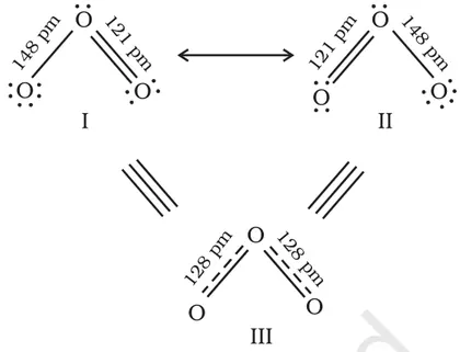
Resonance: When more than one valid Lewis structure exists (differing only in placement of electrons), the true structure is a resonance hybrid. Example: ozone (O3) has two major resonance forms; bond order between terminal and central O is 1.5.
Exceptions to the octet rule:
- Incomplete octet: e.g., BF3 (B has 6 electrons).
- Expanded octet: elements in period 3 and beyond can have >8 e− around central atom (e.g., SF6, PCl5).
- Odd-electron species: free radicals such as NO or NO2 (have unpaired electrons).
Coordinate (dative) covalent bond: A bond in which one atom supplies both electrons of the shared pair (e.g., formation of NH4+ when NH3 donates a lone pair to H+). In final Lewis structures, coordinate bonds are usually drawn as normal covalent bonds but may be indicated with an arrow when showing formation.
Bond order, bond length and bond energy: Higher bond order (single < double < triple) corresponds to shorter bond length and higher bond energy (stronger bond). For resonance structures, the effective bond order is an average (e.g., in benzene, C–C bond order = 1.5).
Importance: Covalent bonding and Lewis structures are foundational for understanding molecular geometry, polarity, reactivity, biochemical interactions, materials, and many applications like drug design, polymer chemistry and material science.
- H2: H–H. Each H shares one electron pair (duet) — single covalent bond.
- Cl2: Cl–Cl. Single covalent bond; each Cl has three lone pairs and completes octet.
- H2O: O with two single bonds to H and two lone pairs; molecular shape = bent (104.5°).
- CO2: O=C=O. Central C makes two double bonds; molecule is linear and nonpolar.
- O3 (ozone): Two resonance forms (one single + one double bond each); average bond order = 1.5; formal charges present.
- NH4+: Formed when NH3 donates a lone pair to H+ (dative bond in formation). Final structure has four equivalent N–H bonds and positive charge on N.
- Formal charge: FC = V − N_nonbonding − 1/2 N_bonding (V = valence electrons of atom).
- Bond order (simple/resonance average): bond order = (total number of bonds between two atoms across resonance structures) / (number of resonance structures) — e.g., O3 central-to-terminal bond order = (1+2)/2 = 1.5.
- Relationship (qualitative): Bond order ∝ bond energy and ∝ 1/(bond length). Higher bond order → shorter and stronger bond.
- Total valence electrons (for drawing Lewis): Sum of valence electrons of all atoms ± electrons for ion charge.
Resonance and Resonance Energy
Definition: Resonance is a way of describing the electronic structure of molecules in which a single Lewis structure cannot adequately represent the observed bonding. Instead, several contributing (canonical) structures are written; the actual structure (the resonance hybrid) is a delocalized blend of these contributors.
Key points:
- Only the positions of electrons (π electrons and lone pairs) change between resonance forms; the positions of atoms remain the same.
- Use a double-headed arrow (<=>) between resonance forms to show they are contributors, not isomers.
- The resonance hybrid is more stable than any single contributing structure because of electron delocalization.
- Major contributors have (in descending importance): complete octets for second-row atoms, minimal charge separation, negative formal charge on the more electronegative atom, and greater covalent character.
Resonance hybrid and bond properties: In the resonance hybrid, bond orders, bond lengths, and charge distributions are intermediate between those in contributing structures. For example, all C–C bonds in benzene are equal and intermediate between single and double bonds.
Resonance energy (stabilization due to resonance): Resonance energy (RE) is the extra stabilization gained by the real (delocalized) molecule compared to the most stable plausible localized structure. It can be estimated experimentally, often using heats of hydrogenation or formation.
Common experimental approach (hydrogenation method): For conjugated pi systems, compare the measured enthalpy change for hydrogenation of the real molecule (ΔHhyd,obs) with the value expected if the pi bonds were isolated/localized (ΔHhyd,expected).
Interpretation: A positive resonance energy (ΔE or RE) means the actual molecule is more stable (lower in energy) than the localized picture. Resonance often explains unusual stability (aromaticity), acidity/basicity changes, and equalized bond lengths.
Examples of common resonance-stabilized species: benzene (aromatic stabilization), acetate ion (delocalized negative charge over two oxygens), nitrate ion, phenoxide ion, allyl cation/anion/radical.
Practical significance: Resonance explains: aromatic stability (benzene chemistry), acid strengths (carboxylates more stable than alkoxides), reactivity patterns in electrophilic and nucleophilic substitution, stabilization of intermediates (carbocations, radicals) by delocalization.
- Benzene (C6H6): six π electrons delocalized over six carbon atoms. All C–C bonds are equal; resonance energy ~152 kJ mol⁻¹ (from hydrogenation comparison).
- Acetate ion (CH3COO–): two equivalent resonance forms with negative charge delocalized over both oxygens; explains increased stability of carboxylate and acidity of acetic acid.
- Nitrate ion (NO3–): three equivalent resonance forms; charge and bond order are delocalized producing equal N–O bond lengths.
- Phenoxide ion (C6H5O–): negative charge on oxygen delocalized into the aromatic ring (several resonance forms), stabilizing the conjugate base and increasing acidity of phenol relative to alcohols.
- Allyl cation/anion: positive/negative charge delocalized over three carbon atoms, stabilizing the species compared to a localized charge.
- Resonance energy (general concept): RE = E_localized − E_delocalized (energy units, e.g., kJ mol⁻¹).
- Hydrogenation method (common experimental estimate): RE ≈ ΔH_hyd,expected − ΔH_hyd,observed. (For benzene: expected ≈ 3 × (hydrogenation of one C=C) ≈ 3 × 120 kJ mol⁻¹ = 360 kJ mol⁻¹; observed ≈ 208 kJ mol⁻¹; RE ≈ 360 − 208 = 152 kJ mol⁻¹.)
- Alternate energy comparison: RE ≈ ΔH_f,calculated (from localized structures) − ΔH_f,experimental (from real compound).
Exceptions to the Octet Rule
What is the octet rule? The octet rule states that atoms tend to gain, lose or share electrons to obtain eight electrons in their valence shell (like the noble gases). It is a simple guideline useful for many main-group compounds, but there are important, systematic exceptions.
Main classes of exceptions
- Incomplete octet (electron-deficient species)
Some atoms (especially small atoms with few valence electrons) form stable compounds in which the central atom has fewer than eight electrons. Common examples: H (2 e-), He, Li, Be, B. Reason: not enough valence electrons or high energy cost to form extra bonds. Lewis-structure approach: minimize formal charge; often these compounds are stabilized by coordinate bonding, dimerization or by acting as Lewis acids. - Odd-electron species (free radicals)
Molecules with an odd total number of electrons cannot give all atoms an octet. Examples: NO, NO2, ClO2, methyl radical (CH3·). These species are often reactive. Modern treatment uses molecular orbital (MO) theory or radical Lewis structures with an unpaired electron indicated on one atom. - Expanded octet (hypervalent species)
Elements in period 3 and beyond (e.g., P, S, Cl, Xe) can accommodate more than eight electrons around the central atom — commonly 10, 12, or more. Examples: PCl5 (10 e- around P), SF6 (12 e- around S), ClF3 (10 e-). Classical explanation invoked d-orbital participation; modern views prefer resonance/charge-separated structures, three-center four-electron bonding, and valence bond / molecular orbital descriptions. The ability to expand the valence shell arises because available orbitals and energetic factors allow more electron density around larger central atoms.
Why do these exceptions occur?
- Small atoms (B, Be) lack sufficient valence electrons and/or orbitals to achieve eight electrons without paying a large energy cost.
- Odd-electron species simply have an odd total electron count determined by constituent atoms (molecular orbital theory explains the single unpaired electron).
- Heavier atoms (period >=3) can accommodate extra electron density because their valence shell is spatially larger; resonance and multicenter bonding often stabilize expanded configurations.
How to handle exceptions in practice (Lewis/MO rules)
- Draw Lewis structures and calculate formal charges to find the most reasonable structure. For electron-deficient molecules, expect positive formal charge on the central atom and consider dimerization or acceptor behavior.
- For radicals, place the unpaired electron on the atom predicted by electronegativity and resonance stabilization; use MO theory for bond order and magnetic properties.
- For hypervalent molecules, allow expanded octet for period-3+ central atoms; check alternative descriptions using resonance forms and three-center bonds to explain bonding without invoking d-orbital participation explicitly.
Practical considerations / stability
- Electron-deficient species are often strong Lewis acids (e.g., BF3 accepts an electron pair).
- Radicals are generally reactive and short-lived, though some (like NO) are stabilized by resonance or delocalization.
- Hypervalent species can be quite stable (SF6 is chemically inert and used industrially), but reactivity depends on both electronic and steric factors.
Summary The octet rule is a useful first approximation but fails for electron-deficient molecules, radicals (odd-electron species), and hypervalent molecules. Modern bonding theories (valence bond, MO theory, and resonance) explain these exceptions without relying solely on the simple octet concept.
- Incomplete octet: BF3 (boron has 6 electrons); BeCl2 (linear, Be has 4 electrons); AlCl3 (often exists as Al2Cl6 dimer to reduce electron deficiency).
- Odd-electron species (radicals): NO (11 valence electrons, paramagnetic), NO2 (one unpaired electron, resonant structures), CH3· (methyl radical in combustion chemistry).
- Expanded octet (hypervalent): PCl5 (phosphorus has 10 valence electrons), SF6 (sulfur has 12 valence electrons, used as an insulating gas in electrical equipment), ClF3 and SF4 (three-center bonding and lone pairs influence geometry).
- Total valence electrons = sum of valence electrons of all atoms (take into account ionic charges if present).
- Formal charge (FC) = V - (N_nonbonding + 1/2 N_bonding), where V = valence electrons for the free atom.
- Electrons around an atom in a Lewis structure = N_nonbonding + 2*(number of bonds to that atom). Use this to check octet (8) or detect exceptions.
- Example electron count checks: BF3 → B: 3 bonds → electrons around B = 2*3 = 6 (incomplete octet). SF6 → S: 6 bonds → electrons around S = 2*6 = 12 (expanded octet). NO (11 e-) → impossible to give all atoms an octet; one unpaired electron remains.
Bond Parameters
Bond parameters are measurable features that describe the nature, strength and geometry of a chemical bond. The main bond parameters studied in Class 11 are bond length, bond angle, bond energy (bond enthalpy or dissociation energy), bond order and bond polarity/dipole moment. These parameters determine molecular shape, stability, reactivity and many physical properties.
1. Bond length (r or r_e)
Bond length is the equilibrium distance between the nuclei of two bonded atoms. It is usually expressed in picometres (pm) or angstroms (Å) (1 Å = 100 pm). Bond length depends on the sizes of the atoms, bond order (single > double > triple in decreasing length), hybridisation (sp < sp2 < sp3), and electronegativity differences. Typical examples: C–C single ≈ 154 pm, C=C ≈ 134 pm, C≡C ≈ 120 pm, H–H ≈ 74 pm.
2. Bond angle (θ)
Bond angle is the angle between two bonds originating from the same atom. It is determined by electron-pair repulsion (VSEPR) and hybridisation: tetrahedral (sp3) ≈ 109.5°, trigonal planar (sp2) ≈ 120°, linear (sp) = 180°. Lone pairs reduce bond angles (e.g., NH3 ≈ 107°, H2O ≈ 104.5°).
3. Bond energy (D or D0)
Bond energy (bond enthalpy) is the energy required to break one mole of bonds in gaseous molecules to give separated atoms (units: kJ·mol−1). It reflects bond strength. Higher bond order generally means higher bond energy. Examples: H–H ≈ 436 kJ·mol−1, C–H ≈ 413 kJ·mol−1, C=C ≈ 614 kJ·mol−1, C≡C ≈ 839 kJ·mol−1. Bond energy varies with molecular environment, so tabulated values are averages.
4. Bond order
Bond order is the number of chemical bonds between a pair of atoms. In valence-bond and resonance contexts it can be a fractional value (e.g., benzene C–C bond order = 1.5). In Molecular Orbital (MO) theory: Bond order = (number of electrons in bonding MOs − number in antibonding MOs)/2. Higher bond order → shorter and stronger bonds.
5. Bond polarity and dipole moment (μ)
If bonded atoms have different electronegativities, the bond is polar and a dipole moment arises. Dipole moment μ = Q × r (charge separation × distance) and is measured in Debye (1 D ≈ 3.336 × 10⁻³⁰ C·m). The molecular dipole moment depends on both bond dipoles and molecular geometry (e.g., CO2 has polar bonds but zero net dipole because it is linear).
6. Potential energy curve and equilibrium
A typical potential energy vs internuclear distance curve shows a minimum at the equilibrium bond length r_e. The well depth (D_e) is the dissociation energy (excludes zero-point energy). Near the minimum the potential is approximately harmonic and vibrations follow Hooke-like behaviour.
Factors affecting bond parameters include atomic size, bond order, electronegativity difference, hybridisation, resonance (delocalisation), formal charge and steric/electronic effects from neighbouring groups.
Practical importance: Bond parameters explain why some bonds are strong (N≡N in nitrogen gas) and inert, why water is polar and has high boiling point (O–H polarity + hydrogen bonding), why double bonds restrict rotation (important in organic stereochemistry) and why fuels release energy (breaking and forming bonds during combustion).
- Water (H2O): O–H bond length ≈ 96 pm, bond angle ≈ 104.5°; strong polarity leads to hydrogen bonding and high boiling point.
- Ethane vs Ethene vs Ethyne: C–C lengths ~154 pm (single), ~134 pm (double), ~120 pm (triple); higher bond order → shorter and stronger bonds.
- Carbon dioxide (CO2): two polar C=O bonds but linear geometry → net dipole = 0 (molecule is nonpolar).
- Benzene (C6H6): resonance gives C–C bond order 1.5 and equal bond lengths (~140 pm) between single and double values.
- Nitrogen gas (N≡N): triple bond very short and very strong (bond dissociation energy ≈ 945 kJ·mol−1), explaining N2 inertness at room temperature.
- Bond order (MO theory) = (electrons in bonding MOs − electrons in antibonding MOs) / 2
- Dipole moment: μ = Q × r (Q = magnitude of partial charge, r = distance between charges); units: Debye (1 D = 3.336×10⁻³⁰ C·m)
- Approximate vibrational frequency (harmonic oscillator): ν = (1 / 2πc) × sqrt(k / μ_red) where k = force constant, μ_red = reduced mass, c = speed of light
- Relation (qualitative): higher bond order → shorter bond length and greater bond energy (no single universal algebraic formula linking length and energy; trends are used)
- Conversion: 1 Å = 100 pm
Polarity of Bonds and Molecules
Overview
Polarity of bonds and molecules describes how electrical charge is distributed in a chemical bond or across a whole molecule. It arises from differences in electronegativity (ability of an atom to attract electrons) between bonded atoms and from the three‑dimensional arrangement of bonds.
Bond Polarity (Bond Dipole)
When two atoms with different electronegativities form a covalent bond, the shared electron pair is displaced toward the more electronegative atom. This creates a partial negative charge (δ–) on the more electronegative atom and a partial positive charge (δ+) on the other. The separation of charge creates a bond dipole, represented by a vector μ (arrow pointing to δ– with a plus sign at the tail).
Dipole Moment (μ)
Dipole moment is a quantitative measure of bond polarity. It is defined as:
μ = q × r
where q is the magnitude of charge separation and r is the distance between charges. μ is a vector (has magnitude and direction). In SI units μ is in coulomb·metre (C·m); chemists commonly use the Debye (D): 1 D = 3.33564 × 10⁻³⁰ C·m.
Electronegativity and Types of Bonds (approximate CBSE guideline)
- Δχ = 0 − 0.4: essentially nonpolar covalent
- Δχ = 0.4 − 1.7: polar covalent
- Δχ > 1.7: predominantly ionic (partial/complete electron transfer)
Percent Ionic Character (Pauling relation)
Pauling proposed an empirical relation to estimate ionic character from electronegativity difference Δχ = |χA − χB|:
% ionic character ≈ [1 − exp(−0.25 × (Δχ)²)] × 100%
Molecular Polarity
A molecule's net polarity depends on the vector sum of all bond dipoles and any lone-pair contribution. If the bond dipoles cancel by symmetry, the molecule is nonpolar even if individual bonds are polar. If they do not cancel, the molecule is polar and has a net dipole moment.
Common geometry examples
- CO₂ (linear): two equal C=O bond dipoles are opposite → net μ = 0 → nonpolar.
- H₂O (bent, 104.5°): bond dipoles do not cancel → net μ ≠ 0 → polar (μ ≈ 1.85 D).
- NH₃ (trigonal pyramidal): lone pair and bond dipoles give a net dipole → polar (μ ≈ 1.47 D).
- BF₃ (trigonal planar): three identical B–F dipoles cancel → nonpolar.
- CH₄, CCl₄ (tetrahedral with identical substituents): dipoles cancel → nonpolar.
- HCl (diatomic, Δχ large): polar covalent with a clear dipole (δ+ on H, δ– on Cl).
- NaCl (solid): essentially ionic lattice with full charge separation in formula unit.
Consequences and Real‑life relevance
Polarity explains many physical properties and phenomena: high boiling point and surface tension of water (hydrogen bonding), solubility rules (“like dissolves like”), behavior of solvents (polar vs nonpolar), dipole‑dipole interactions in liquids and solids, dielectric constants, molecular recognition in biology (enzyme–substrate, membrane transport), design of drugs and materials.
How to decide molecular polarity (stepwise)
1. Draw the Lewis structure and determine molecular geometry (VSEPR).
2. Determine bond polarities from electronegativity differences and draw bond dipole vectors.
3. Vectorially add dipoles (consider magnitude and direction) to find net dipole moment.
4. If net μ ≠ 0 → molecule is polar; if net μ = 0 → nonpolar.
Experimental measure
Dipole moments can be measured by dielectric constant and microwave spectroscopy. Values are tabulated for many molecules (units in Debye).
Simple visual aids to use in class
- Vector arrows on 2D/3D ball‑and‑stick models showing bond dipoles and resultant μ.
- Electron density maps (schematic) showing charge accumulation on the more electronegative atom.
- Comparison of polar vs nonpolar solvents and examples of solubility (e.g., oil in water vs oil in hexane).
- HCl: Polar diatomic molecule — Cl is more electronegative, so Hδ+—Clδ–; dipole moment ≈ 1.08 D.
- H2O: Bent geometry causes two O–H bond dipoles to add to a net dipole (μ ≈ 1.85 D) → polar; explains high boiling point and hydrogen bonding.
- CO2: Linear geometry with two equal C=O bond dipoles in opposite directions → net μ = 0 → nonpolar despite polar bonds.
- BF3: Trigonal planar; three equal B–F bond dipoles cancel → nonpolar; used to illustrate symmetry causing cancellation.
- NaCl: Large electronegativity difference → primarily ionic compound (crystalline lattice of Na+ and Cl–).
- CH4 and CCl4: Tetrahedral molecules with symmetric substituents → individual bond dipoles cancel → nonpolar.
- Dipole moment: μ = q × r (q = charge magnitude, r = distance between charges).
- Unit conversion: 1 Debye (D) = 3.33564 × 10⁻³⁰ C·m.
- Pauling % ionic character: % ionic ≈ [1 − exp(−0.25 × (Δχ)²)] × 100%, where Δχ = |χA − χB|.
- Electronegativity-based classification (approximate): Δχ = 0–0.4 nonpolar covalent; 0.4–1.7 polar covalent; >1.7 ionic.
Valence Shell Electron Pair Repulsion (VSEPR) Theory
What is VSEPR?
VSEPR (Valence Shell Electron Pair Repulsion) theory explains the shapes of molecules by assuming that electron pairs (bonding and lone pairs) around a central atom repel one another and thus arrange themselves as far apart as possible in 3‑D space. The arrangement of these electron domains determines molecular geometry.
Basic principles
- Count electron domains (regions of electron density) around the central atom: each lone pair, each single bond, and each multiple bond counts as one domain.
- Electron domains arrange to minimize repulsion — this gives the electron‑domain geometry (ideal geometry if only positions of electron domains are considered).
- The actual molecular shape (positions of atoms) is obtained by placing atoms on those domain positions; lone pairs are not shown as atoms but affect bond angles.
- Repulsion strength order: lone pair–lone pair (LP–LP) > lone pair–bonding pair (LP–BP) > bonding pair–bonding pair (BP–BP). Lone pairs compress bond angles between bonded atoms.
- Multiple bonds (double, triple) count as one domain but exert slightly greater repulsion than a single bond.
Steps to predict molecular shape (concise)
- Identify the central atom (usually least electronegative or the one with most bonds).
- Draw the Lewis structure and count lone pairs on the central atom.
- Compute the steric number (SN) = number of sigma bonds on central atom + number of lone pairs = number of electron domains.
- Use SN to find electron geometry (SN 2→linear, 3→trigonal planar, 4→tetrahedral, 5→trigonal bipyramidal, 6→octahedral).
- Adjust to molecular geometry by placing atoms and accounting for lone pairs (which reduce bond angles).
Common geometries and typical bond angles
- SN = 2: linear, bond angle 180° (example: CO2).
- SN = 3: trigonal planar, 120°; with 1 LP → bent (~<120°) (example: BF3; SO2).
- SN = 4: tetrahedral 109.5°; with 1 LP → trigonal pyramidal (~107°) (NH3); with 2 LP → bent (~104.5°) (H2O).
- SN = 5: trigonal bipyramidal (axial 90°, equatorial 120°); with 1 LP → seesaw; 2 LP → T‑shaped; 3 LP → linear (example: PF5, SF4, ClF3, I3−).
- SN = 6: octahedral 90°; with 1 LP → square pyramidal; with 2 LP (opposite) → square planar (example: SF6, XeF4).
Limitations and notes
- VSEPR predicts geometry qualitatively; small deviations occur due to differences in electronegativity, lone‑pair orbital character, and multiple‑bond repulsion being slightly larger.
- For molecules with expanded octets (period 3 and beyond), VSEPR still applies using domain count but consider d‑orbital involvement only historically — modern explanations use electron domain minimization without invoking d‑orbitals explicitly.
- Resonance can affect apparent lone‑pair distribution; use averaged structures for geometry predictions.
- CO2 — Linear (SN=2). Carbon has two double bonds; electron domains = 2 → 180°. Real‑life: major greenhouse gas.
- BF3 — Trigonal planar (SN=3). Three B–F bonds, no lone pair → 120°. Real‑life: Lewis acid used in organic synthesis.
- CH4 — Tetrahedral (SN=4). Four single bonds → 109.5°. Real‑life: methane is main component of natural gas.
- NH3 — Trigonal pyramidal (SN=4 with 1 LP). One lone pair compresses H–N–H to ~107°. Real‑life: ammonia in fertilizers and cleaning agents.
- H2O — Bent (SN=4 with 2 LP). Two lone pairs compress H–O–H to ~104.5°. Real‑life: water’s bent shape gives polarity and hydrogen bonding, crucial for life.
- PF5 — Trigonal bipyramidal (SN=5). Two axial (90° to equatorial) and three equatorial (120° between them). Real‑life: example of molecules with different axial/equatorial bond environments.
- AXE notation: A = central atom, X = number of bonded atoms, E = number of lone pairs on A. Example: CH4 = AX4, NH3 = AX3E, H2O = AX2E2.
- Steric number (SN) = number of sigma bonds on central atom + number of lone pairs on central atom. SN determines electron‑domain geometry.
- Electron‑domain count rule: each single bond, each multiple bond, and each lone pair count as one domain.
- Repulsion order (qualitative inequality): LP–LP > LP–BP > BP–BP (used to predict bond angle deviations).
Molecular Shapes (VSEPR Examples)
VSEPR principle (Valence Shell Electron Pair Repulsion): The shape of a molecule is determined by repulsions between electron domains (bonding pairs and lone pairs) around the central atom. Electron domains arrange themselves to minimize repulsion, giving characteristic geometries.
Key concepts and steps to predict shape:
- Count valence electrons and draw the Lewis structure.
- Determine the number of electron domains (steric number) around the central atom: steric number = number of bonded atoms + number of lone pairs.
- Use the VSEPR notation AXnEm (A = central atom, X = bonded atoms, E = lone pairs) to identify the electron-domain geometry (arrangement of all domains) and molecular geometry (positions of atoms only).
- Account for lone pair effects: lone pairs occupy more space and repel bonding pairs, reducing bond angles.
Electron pair repulsion order: LP–LP > LP–BP > BP–BP (LP = lone pair, BP = bonding pair). This explains why bond angles decrease as lone pairs increase.
Common geometries (brief): linear (SN=2), trigonal planar (SN=3), bent (from trigonal planar SN=3 with 1 lone pair), tetrahedral (SN=4), trigonal pyramidal (SN=4 with 1 lone pair), bent (SN=4 with 2 lone pairs), trigonal bipyramidal (SN=5), seesaw/T-shaped/linear (variants for SN=5 with lone pairs), octahedral (SN=6), square pyramidal and square planar (variants for SN=6 with lone pairs).
Effect on bond angles: For SN=4 (electron geometry tetrahedral): ideal angle 109.5°. With one lone pair (trigonal pyramidal like NH3) angle ≈ 107°, with two lone pairs (bent like H2O) angle ≈ 104.5°. Similar reductions occur for other steric numbers.
Limitations: VSEPR is an effective, simple model for main-group molecules but does not explicitly include effects of multiple bonds (which act like more than one electron domain), d-orbital participation in heavy elements, or subtle electronic/steric effects—use molecular orbital or experimental data when needed.
- CO2 — linear (AX2): central C has SN = 2; bond angle = 180°; important greenhouse gas.
- BF3 — trigonal planar (AX3): central B has SN = 3; bond angle = 120°; used in organic catalysis.
- SO2 — bent (AX2E): central S has SN = 3 with one lone pair; bond angle ≈ 119°; pollutant from combustion.
- CH4 — tetrahedral (AX4): central C has SN = 4; bond angle = 109.5°; methane is main component of natural gas.
- NH3 — trigonal pyramidal (AX3E): central N SN = 4 with one lone pair; bond angle ≈ 107°; common household ammonia.
- H2O — bent (AX2E2): central O SN = 4 with two lone pairs; bond angle ≈ 104.5°; water’s shape causes its polarity and many unique properties.
- Steric number (SN) = number of atoms bonded to central atom + number of lone pairs on central atom.
- VSEPR notation: AXnEm (A = central atom, X = bonded atoms, E = lone pairs).
- Hybridization estimate from SN: SN 2 → sp, SN 3 → sp2, SN 4 → sp3, SN 5 → sp3d, SN 6 → sp3d2 (use as guideline).
- Order of repulsion strength: LP–LP > LP–BP > BP–BP.
- Approximate bond angles: linear 180°; trigonal planar 120°; tetrahedral 109.5°; trigonal bipyramidal 90°/120°; octahedral 90°.
Valence Bond Theory (VBT)
Definition: Valence Bond Theory (VBT) explains covalent bond formation as the result of overlap between half‑filled atomic orbitals of two atoms, with the sharing of a pair of electrons of opposite spins. VBT emphasises the directional nature of covalent bonds and introduces the idea of hybridisation to explain molecular shapes.
Key postulates:
- A covalent bond forms when two half‑filled atomic orbitals (one from each atom) overlap and their unpaired electrons pair with opposite spins.
- The extent of overlap determines bond strength and bond length: greater overlap → stronger, shorter bond.
- Overlaps along the internuclear axis produce σ (sigma) bonds; sidewise overlaps of parallel p‑orbitals produce π (pi) bonds.
- Atomic orbitals on the same atom can mix (hybridise) to form equivalent directional hybrid orbitals (sp, sp2, sp3, ...), which better explain molecular geometry.
- Resonance in many molecules is represented in VBT by combining several contributing valence‑bond structures; the real structure is a resonance hybrid.
Types of overlap:
- σ overlap: head‑on overlap (s–s, s–p, p–p along axis). Single bonds are σ bonds.
- π overlap: lateral (side‑by‑side) overlap of unhybridized p orbitals; π bonds accompany σ bonds in double and triple bonds (double = 1σ + 1π, triple = 1σ + 2π).
Hybridisation (VBT treatment): To explain molecular shapes, atomic orbitals mix to give directional hybrid orbitals. The simplest rule: number of electron‑regions (σ bonds + lone pairs) around central atom = number of hybrids.
- 2 regions → sp (linear, 180°)
- 3 regions → sp2 (trigonal planar, 120°)
- 4 regions → sp3 (tetrahedral, 109.5°)
- 5 regions → sp3d (trigonal bipyramidal)
- 6 regions → sp3d2 (octahedral)
How VBT describes common molecules (brief):
- H2: overlap of two 1s orbitals (σ bond).
- Cl2: overlap of two 3p orbitals along axis (σ from p–p).
- CH4: C undergoes sp3 hybridisation; four sp3 orbitals overlap with four H 1s orbitals → four σ bonds (tetrahedral).
- C2H4 (ethylene): each C is sp2 hybridised (three sp2 form σ bonds); remaining unhybridised p on each C overlap side‑by‑side → one π bond; molecule is planar.
- C2H2 (acetylene): C is sp hybridised; two unhybridised p orbitals on each C form two π bonds (triple bond overall).
Strengths of VBT:
- Explains directional nature and shapes of molecules via hybridisation.
- Qualitatively describes σ and π bonding and bonding in organic molecules.
- Useful for drawing Lewis structures with orbital pictures.
Limitations:
- VBT cannot easily explain spectroscopic energy levels and magnetic properties for some molecules (e.g., it struggles to predict the paramagnetism of O2 accurately — MO theory does better).
- Quantitative predictions of bond energies and electron distributions are limited compared with Molecular Orbital (MO) theory.
Summary: VBT views covalent bonding as overlap of atomic orbitals with pairing of opposite‑spin electrons; hybridisation is used to explain molecular geometry and equivalent bonds. It is a simple, visual model widely used in Class 11/12 chemistry, especially for organic molecules, but has known limitations where MO theory is required.
- H2: 1s–1s head‑on overlap → σ bond (simple example of bond formation).
- Cl2: p–p head‑on overlap of two chlorine 3p orbitals forming a σ bond.
- CH4 (methane, natural gas component): C is sp3 hybridised; four sp3 orbitals overlap with 4 H 1s → tetrahedral molecule (109.5°).
- C2H4 (ethylene, used as plant hormone and in polymer production): each C is sp2 hybridised; one σ and one π bond between carbons (planar molecule).
- C2H2 (acetylene, used as welding fuel): C is sp hybridised; triple bond (1σ + 2π) between carbons — linear molecule.
- NH3 (ammonia, fertiliser precursor): N is sp3 hybridised with one lone pair; lone pair‑bond pair repulsion reduces H–N–H angle (~107°).
- Overlap integral (measure of overlap): S = ∫ φ_A(r) φ_B(r) dτ (qualitative: larger S → stronger bond).
- Hybridisation rule (number of electron regions = number of hybrids): 2 → sp, 3 → sp2, 4 → sp3, 5 → sp3d, 6 → sp3d2.
- Condition for covalent bond (VBT statement): two half‑filled orbitals from different atoms + opposite electron spins → bond formation.
- Bond types (VBT count): single bond = 1 σ, double bond = 1 σ + 1 π, triple bond = 1 σ + 2 π.
- \[(Optional/related) Pauling estimate of % ionic character: % ionic ≈ [1 − e^{−(Δχ)^2/4}] × 100%\]\[where Δχ = difference in Pauling electronegativities.\]
Hybridisation
What is hybridisation?
Hybridisation is a model in valence bond theory that explains the formation of equivalent directional orbitals (hybrid orbitals) by mixing atomic orbitals (AOs) of comparable energy on the same atom. These hybrid orbitals then form sigma (σ) bonds or hold lone pairs, giving rise to observed molecular shapes and bond angles.
Why is it used?
Atomic s and p orbitals have different shapes and energies. To explain observed molecular geometries (e.g., tetrahedral CH4, trigonal planar BF3), we imagine that atomic orbitals mix to produce new equivalent orbitals oriented to minimize electron-pair repulsion.
How hybrid orbitals are formed
- The number of hybrid orbitals equals the number of atomic orbitals mixed.
- The energy of hybrid orbitals lies between the energies of the original atomic orbitals.
- The orientation of hybrid orbitals is such that electron-pair repulsion is minimized (gives observed geometry).
Common types, geometry and bond angles
| Steric number (no. of σ bonds + lone pairs) | Hybridisation | Geometry | Ideal bond angles |
|---|---|---|---|
| 2 | sp | Linear | 180° |
| 3 | sp2 | Trigonal planar | 120° |
| 4 | sp3 | Tetrahedral | 109.5° |
| 5 | sp3d | Trigonal bipyramidal | 90°, 120° |
| 6 | sp3d2 | Octahedral | 90° |
Determining hybridisation (practical steps)
1. Choose the central atom.
2. Count the number of atoms directly bonded to it (each single, double, triple bond counts as one sigma).
3. Count lone pairs on the central atom.
4. Steric number = (number of bonded atoms) + (number of lone pairs).
5. Use the steric number to assign hybridisation from the table above.
S-character and its consequences
s-character = (number of s AOs in hybrid / total number of AOs mixed) × 100. For example: sp3 → 25% s-character, sp2 → 33.3%, sp → 50%.
Higher s-character means electrons are held closer to the nucleus, which leads to (a) shorter and stronger bonds, and (b) greater acidity of a C–H bond (hence alkynes > alkenes > alkanes in acidity).
Lone pairs and bond angles
Lone pairs occupy hybrid orbitals and repel bonding pairs more strongly, reducing bond angles (e.g., NH3 ≈ 107° and H2O ≈ 104.5° instead of 109.5° for ideal sp3).
Limitations & remarks
- Hybridisation is a useful approximation; molecular orbital (MO) theory gives a more complete quantum description.
- For some molecules (especially with delocalised π systems like benzene), hybridisation must be combined with the concept of delocalised π MOs (benzene C atoms are sp2 and each contributes a p orbital to a delocalised π system).
- For elements of period 3 and beyond, d-orbitals may participate (sp3d, sp3d2) to accommodate expanded coordination, though modern descriptions sometimes describe these cases with MO or three-center bonding models.
- Methane (CH4): Carbon is sp3 hybridised → 4 equivalent sp3 orbitals form 4 σ C–H bonds; geometry tetrahedral, bond angle ≈ 109.5°.
- Ethene (C2H4): Each carbon is sp2 hybridised → 3 sp2 orbitals make σ bonds (two C–H and one C–C), remaining unhybridised p orbital forms a π bond; geometry trigonal planar, bond angles ≈ 120°.
- Ethyne (C2H2): Each carbon is sp hybridised → 2 sp orbitals form σ bonds (one C–H and one C–C), two unhybridised p orbitals form two π bonds (triple bond); geometry linear, bond angle 180°.
- Benzene (C6H6): Each carbon is sp2; one unhybridised p orbital on each C forms a delocalised π system, giving planar hexagonal structure.
- Water (H2O): Oxygen is sp3 hybridised; two lone pairs occupy two sp3 orbitals producing bent geometry (≈104.5°).
- Phosphorus pentachloride (PCl5): P in the central atom is often described as sp3d hybridised → trigonal bipyramidal geometry (90° & 120°).
- Steric number = (number of σ bonds to central atom) + (number of lone pairs on central atom)
- Number of hybrid orbitals = number of atomic orbitals mixed (equals steric number)
- s-character (%) = (number of s orbitals in hybrid / total orbitals mixed) × 100. Examples: sp3 → 1/4 = 25%, sp2 → 1/3 ≈ 33.3%, sp → 1/2 = 50%
- Typical bond angle approximations: sp → 180°, sp2 → 120°, sp3 → 109.5°, sp3d → 90° & 120°, sp3d2 → 90°
- Correlation (qualitative): greater s-character → shorter bond length, higher bond strength, greater acidity of attached H (pKa trend: sp H < sp2 H < sp3 H)
Sigma and Pi Bonds
Introduction & definitions
Chemical bonds between atoms arise from overlap of atomic orbitals. Sigma (σ) and pi (π) bonds are two fundamental types of covalent overlap:
- Sigma bond (σ): Formed by head-on (axial) overlap of orbitals (s–s, s–p, p–p (end-to-end) or hybrid orbitals). The electron density is concentrated along the internuclear axis. A single covalent bond is always one σ bond.
- Pi bond (π): Formed by side-by-side (lateral) overlap of two parallel unhybridized p orbitals. Electron density is concentrated above and below (or in front and behind) the internuclear axis and there is a nodal plane containing the internuclear axis where electron density is zero.
Formation & orbital requirements
σ bonds come from end-to-end overlap; they can involve hybrid orbitals (sp3, sp2, sp) or s orbitals. π bonds always involve unhybridized p orbitals remaining after hybridization:
- sp3 C: 4 σ bonds (no π)
- sp2 C: 3 σ bonds + 1 unhybridized p → can form 1 π (as in C=C)
- sp C: 2 σ bonds + 2 unhybridized p → can form 2 π (as in C≡C)
Characteristics & comparison
- Symmetry: σ bond is cylindrically symmetric about the bond axis; π bond has a nodal plane along the bond axis.
- Strength & overlap: σ overlap (end-to-end) is generally greater than π (side-by-side), so σ bonds are stronger and shorter than a single π contribution between the same atoms.
- Rotation: Single σ bonds allow free rotation about the bond axis (ignoring steric/electronic effects). Presence of a π bond (as in double bonds) restricts rotation due to the need to maintain p–p overlap.
- Reactivity: π electrons are more exposed and thus more chemically reactive (sites for electrophilic addition, e.g., alkenes) compared to σ electrons.
Relation to single, double and triple bonds
A single bond = 1σ. A double bond = 1σ + 1π. A triple bond = 1σ + 2π. More π bonds increase bond order (and shorten/strengthen the bond) but each additional π is usually weaker than the σ.
Molecular orbital (MO) perspective (brief)
In MO theory, σ and π refer to symmetry of MOs about the molecular axis. Bonding MOs (σ, π) are lower in energy; antibonding MOs are σ* and π*. Bond order (MO) = 1/2 (number of electrons in bonding MOs − number in antibonding MOs). Example: in N2 the triple bond corresponds to filled σ and π bonding MOs giving bond order 3.
Why hybridization matters
Hybrid orbitals form σ bonds and determine molecular geometry (sp3 → tetrahedral, sp2 → trigonal planar, sp → linear). The remaining unhybridized p orbitals form π bonds when parallel.
Summary
σ = head-on overlap, stronger, allows rotation; π = side-on overlap, weaker per overlap, restricts rotation and is chemically reactive. Single = σ only; double = σ+π; triple = σ+2π.
- H2: single σ bond formed by overlap of two 1s orbitals.
- Cl2, F2: single σ bond from p–p (end-to-end) or p–p/s–p interactions depending on orbitals.
- Ethane (C2H6): C–C single bond = one σ (sp3–sp3) → free rotation about C–C.
- Ethene (C2H4): C=C double bond = one σ (sp2–sp2) + one π (side-by-side p–p) → planar, no free rotation.
- Ethyne/Acetylene (C2H2): C≡C triple bond = one σ (sp–sp) + two π (two orthogonal p–p overlaps) → linear.
- Benzene (C6H6): delocalized π system above and below the ring (conjugation) responsible for aromatic stability and many optical/chemical properties.
- Symbol notation: σ (sigma), π (pi), σ* (sigma antibonding), π* (pi antibonding).
- Bond composition: Single = 1σ; Double = 1σ + 1π; Triple = 1σ + 2π.
- MO bond order: bond order = 1/2 (N_bonding − N_antibonding). Example: N2 → bond order = 1/2 (10 − 4) = 3.
- Qualitative relations: greater overlap → stronger bond; higher bond order → shorter bond length and higher bond energy (qualitative).
Molecular Orbital Theory (MOT) — Principles
What is MOT?
Molecular Orbital Theory (MOT) explains bonding in molecules by combining atomic orbitals (AOs) of all atoms to form molecular orbitals (MOs) that extend over the entire molecule. Electrons occupy these MOs; bonding properties result from the distribution of electrons in bonding and antibonding MOs.
Basic principles / steps to form MOs
- Atomic orbitals from the atoms combine to form molecular orbitals. The number of MOs formed equals the total number of combining AOs.
- Two types of combinations: constructive (in-phase) → bonding MO (lower in energy); destructive (out-of-phase) → antibonding MO (higher in energy, often denoted with an asterisk, •*).
- MOs are filled with electrons according to Aufbau principle (low to high energy), Pauli exclusion principle (max two electrons with opposite spins per MO), and Hund’s rule (place unpaired electrons in degenerate orbitals first).
- Only AOs with appropriate symmetry and significant energy overlap combine effectively (same symmetry about the molecular axis; comparable energies; good spatial overlap).
- MOs are classified by their symmetry about the internuclear axis: sigma (σ) — end-on overlap, cylindrical symmetry; pi (π) — side-on overlap, with nodal plane along the axis. For homonuclear diatomics, gerade (g) and ungerade (u) labels indicate symmetry through the center.
Key consequences
- Bond order (a measure of bond strength and stability) = (number of electrons in bonding MOs − number in antibonding MOs) / 2. Higher bond order → shorter, stronger bond.
- Magnetic properties follow occupancy of MOs: molecules with unpaired electrons are paramagnetic; all electrons paired → diamagnetic.
- Relative ordering of 2p MOs: for lighter homonuclear diatomics (B2, C2, N2) the π(2p) MOs lie lower than σ(2p); for O2, F2 and beyond, σ(2p) lies below π(2p). (This affects electronic configuration and properties.)
Examples of application
- H2: two 1s AOs form one bonding σ(1s) and one antibonding σ*(1s); two electrons occupy σ(1s) → bond order = 1.
- He2: four electrons would fill σ(1s) and σ*(1s) equally → bond order = 0 → no stable He2 in normal conditions.
- O2: electronic configuration ends with two unpaired electrons in degenerate π*(2p) MOs → paramagnetic with bond order = 2.
Why MOT is useful
MOT explains bond strengths, bond orders, magnetic behaviour (e.g., O2 paramagnetism), and delocalization (e.g., conjugated pi systems) more naturally than simple valence-bond pictures for many molecules and ions.
Limitations (brief)
MOT can be qualitative without computational methods for complex molecules; orbital energies and exact mixing often require calculations.
- H2: Two 1s AOs combine → σ(1s) (bonding) and σ*(1s) (antibonding). With 2 electrons in σ(1s), bond order = (2−0)/2 = 1 (single bond).
- He2: Four electrons fill σ(1s) and σ*(1s) equally → bond order = (2−2)/2 = 0, so He2 is not stable under normal conditions.
- O2: MO configuration has two unpaired electrons in π*(2p) → paramagnetic; bond order = (8 bonding − 4 antibonding)/2 = 2.
- N2: Strong triple bond explained by filled σ(2s), σ*(2s), σ(2p) and π(2p) MOs; bond order = 3 → very strong bond (important in fertilizers, industrial chemistry).
- CO: MO description explains strong bond, polarity and ability of CO to act as a ligand in metal complexes (donation via lone pair and back-bonding into π*).
- Bond order = (Number of electrons in bonding MOs − Number of electrons in antibonding MOs) / 2
- Total number of MOs formed = Total number of combining AOs
- Magnetic moment (spin-only, for n unpaired electrons) μ = √(n(n + 2)) Bohr magneton (BM)
- Pauli exclusion principle: maximum 2 electrons per MO with opposite spins
- Aufbau & Hund rules: fill lower-energy MOs first; for degenerate MOs maximize unpaired electrons with parallel spins
Molecular Orbital Diagrams for Homonuclear Diatomics
What are Molecular Orbitals (MOs)? Molecular orbitals are wave functions that extend over an entire molecule and are formed by linear combination of atomic orbitals (LCAO). For homonuclear diatomic molecules (A2), MOs arise from the combination of identical atomic orbitals on the two atoms. Each pair of combining atomic orbitals gives one bonding MO (lower energy, constructive interference) and one antibonding MO (higher energy, destructive interference).
Constructing MO diagrams (step-by-step):
- 1) Consider valence atomic orbitals of each atom (for period-2 diatomics: 2s and 2p).
- 2) Combine orbitals of the same symmetry and similar energy: s with s (gives σ2s and σ*2s); pz (axis along internuclear line) gives σ2p/σ*2p; px and py (perpendicular) combine to give two degenerate π2p/π*2p orbitals.
- 3) Arrange MO energy levels according to known ordering (see below). Fill electrons (usually valence electrons only) into MOs following Aufbau, Pauli, and Hund rules.
- 4) Calculate bond order and predict magnetic and stability properties.
Key MO energy ordering (period-2 homonuclear diatomics):
- For B2, C2, N2 (significant s–p mixing): σ(2s) < σ*(2s) < π(2p) < σ(2p) < π*(2p) < σ*(2p).
- For O2, F2, Ne2 (s–p mixing negligible): σ(2s) < σ*(2s) < σ(2p) < π(2p) < π*(2p) < σ*(2p).
- Reason for change: s–p mixing occurs when 2s and 2p energies are close (lighter atoms), which raises σ(2s) and lowers σ(2p) relative positions and inverts the order of σ(2p) and π(2p).
Bond order and stability: Bond order (BO) quantifies bond strength and is computed from the number of electrons in bonding (Nb) and antibonding (Na) MOs:
Bond order = (Nb − Na) / 2
Interpretation: BO > 0 indicates a stable bond; BO = 0 indicates no net bond (molecule not stable under normal conditions).
Magnetic behavior: Unpaired electrons in MOs give paramagnetism. The number of unpaired electrons n can be used to estimate the magnetic moment (spin-only):
μ (Bohr magneton) = √(n(n + 2))
HOMO and LUMO: The Highest Occupied Molecular Orbital (HOMO) and Lowest Unoccupied Molecular Orbital (LUMO) control chemical reactivity (electron donation/acceptance). For example, in N2 the HOMO is σ2p (bonding) and in O2 the HOMO is a singly occupied π*2p (antibonding), explaining O2's paramagnetism and reactivity.
Important points to remember:
- Always consider valence electrons when filling MO diagrams for qualitative bonding.
- s–p mixing affects energy ordering only for the lighter period-2 diatomics (B2–N2).
- Bond order gives the number of electron pairs in bonding MOs minus antibonding MOs; higher bond order generally means shorter, stronger bonds.
- H2: 1s orbitals combine to give σ1s (bonding) and σ*1s (antibonding). 2 electrons occupy σ1s → bond order = 1 (stable).
- He2: σ1s and σ*1s are both filled with 2 electrons each → bond order = 0 (no stable molecule under normal conditions).
- Li2: valence 2s orbitals give σ2s occupied, σ*2s empty → bond order = 1 (weak single bond).
- Be2: σ2s and σ*2s both filled → bond order = 0 (not stable as an isolated diatomic).
- B2: valence configuration yields two unpaired electrons in π2p → bond order = 1; paramagnetic.
- C2: MO filling (with s–p mixing) gives bond order = 2 (double bond).
- Bond order = (Number of electrons in bonding MOs − Number of electrons in antibonding MOs) / 2
- Magnetic moment (spin-only) μ = √(n(n + 2)) Bohr magneton, where n = number of unpaired electrons
- Total valence electrons for A2 = 2 × (valence electrons per atom) — use valence electrons (e.g., for period-2: 2s and 2p electrons)
Molecular Orbitals for Heteronuclear Diatomics
What it means
Heteronuclear diatomics are molecules made of two different atoms (e.g., CO, HF, NO). In the molecular orbital (MO) approach these form MOs by linear combination of the two different atomic orbitals (AOs). Because the two AOs usually have different energies (due to different electronegativities and orbital energies), the resulting MOs are asymmetric and often polarized toward the more electronegative atom.
Basic LCAO-MO idea (two‑orbital case)
If χA and χB are the two combining AOs, an MO is written as: ψ = cA·χA + cB·χB. The coefficients cA and cB depend on the AO energies, their overlap and interaction. When AO energies are different, the lower‑energy AO contributes more to the bonding MO and the higher‑energy AO contributes more to the antibonding MO.
Consequences
- Bonding MO is polarized toward the atom with lower AO energy (more electronegative atom).
- Antibonding MO has greater character of the higher‑energy AO (less electronegative atom).
- Partial ionic character: if AO energy difference is large the bond tends toward ionic behaviour (extreme case: LiF).
- Bond order and magnetic properties follow from MO occupancy in the usual way; heteronuclear diagrams must account for unequal AO energies and unequal orbital contributions.
Ordering and mixing
For period‑2 atoms the relative order of σ2p and π2p MOs can change if s–p mixing is significant (as in some homonuclear cases). In heteronuclear cases s–p mixing is usually reduced because the AO energies differ; therefore the MO ordering is often closer to the simple picture where σ2p lies above π2p for atoms with large energy separation.
How to estimate MO character
- Percent contribution of atom A ≈ (cA² / (cA² + cB²)) × 100%.
- Coefficient ratio in the simple two‑level model (qualitative): cA/cB depends on (E − εA) and the interaction integral; if εA ≪ εB then bonding MO is mostly χA.
Bond order and electrons
Bond order (BO) = 1/2 × (number of electrons in bonding MOs − number in antibonding MOs). This formula and MO electron counting give BO for heteronuclear molecules as for homonuclear ones; the difference is that MOs are not equally shared between atoms.
Practical notes for students
- Draw AO energy levels with the more electronegative atom lower in energy.
- Combine orbitals of the same symmetry to form bonding and antibonding MOs; draw MO energy levels closer to the lower AO for bonding and closer to the higher AO for antibonding.
- Use occupancies to find bond order and unpaired electrons (magnetism).
Summary
Molecular orbitals in heteronuclear diatomics are asymmetric because of unequal AO energies. This leads to polar covalent bonds, varying degrees of ionic character, and MOs whose shapes and energies reflect the differing contributions of the two atoms.
- CO (carbon monoxide): 10 valence electrons from C and O combined give a bond order of 3. MOs are polarized with bonding MOs shifted toward O (more electronegative) but the lone‑pair on C gives a small negative charge on carbon; CO binds strongly to metal centres (biologically and industrially).
- HF (hydrogen fluoride): large AO energy difference between H(1s) and F(2p) gives a bonding MO strongly localized on F and strong polarity (near ionic character).
- LiF (lithium fluoride): very large energy difference → almost ionic behaviour; MO picture shows near complete localization of electron density on F.
- NO (nitric oxide): odd‑electron heteronuclear diatomic with 11 valence electrons → bond order 2.5 and paramagnetism (one unpaired electron).
- HCl (hydrogen chloride): bonding MO has more Cl character causing a polar covalent bond with partial negative on Cl and partial positive on H.
- LCAO: ψ = c_A χ_A + c_B χ_B
- Normalization: c_A² + c_B² + 2c_A c_B S = 1 (S = overlap integral; often approximated by neglecting 2c_A c_B S for qualitative work)
- Percent contribution of atom A = (c_A² / (c_A² + c_B²)) × 100%
- Bond order (BO) = 1/2 × (n_bonding − n_antibonding)
- Relative coefficient dependence (qualitative two‑level): c_A / c_B ∝ H_AB / (E − ε_A) where ε_A is AO energy and H_AB is interaction integral (used in secular equations)
Ionic vs Covalent Character and Electronegativity
Electronegativity (χ) is the tendency of an atom in a molecule to attract shared electrons towards itself. The Pauling scale is the most commonly used scale (e.g. H ≈ 2.1, O ≈ 3.5, Cl ≈ 3.0, Na ≈ 0.93, F ≈ 4.0). Electronegativity increases across a period (left to right) and decreases down a group.
Bond types as a continuum: Bonds are not simply ionic or covalent but lie on a continuum determined mainly by the difference in electronegativity between bonded atoms, Δχ = |χA − χB|. Typical classification (approximate):
- Δχ < 0.4: nonpolar covalent
- 0.4 ≤ Δχ ≤ 1.7: polar (polarised) covalent
- Δχ > 1.7: predominantly ionic (often written as ionic)
Quantifying ionic character
- Pauling empirical relation (gives % ionic character from electronegativity difference):
% ionic character ≈ (1 − e−0.25(Δχ)2) × 100 - Dipole-moment method (experimental): percent ionic character = (observed μ / μionic) × 100, where μ is in Debye. For a completely ionic bond μionic = e × r. In convenient units:
μionic (Debye) ≈ 4.80 × r (Å). So percent ionic = μ(observed, D) / (4.80 × r(Å)) × 100.
Fajan's rules — when ionic compounds show covalent character
- Small cation with high positive charge and large, polarizable anion increases covalent character (electron cloud distortion).
- Greater covalent character: cation small & highly charged, anion large & easily polarised, and when difference in electronegativity is not very large.
Physical consequences
- Ionic compounds: high melting/boiling points, hard and brittle, conduct electricity when molten or in aqueous solution (ions mobile), often soluble in polar solvents (e.g., water).
- Covalent compounds: lower melting/boiling points (molecular), do not conduct electricity in general, solubility varies (nonpolar solvents for nonpolar molecules), polar covalent molecules can have dipole interactions and hydrogen bonding.
Important caveats: Electronegativity difference gives only an approximate separation. Many compounds (e.g., AlCl3, ZnCl2) often labelled ionic show significant covalent character due to polarisation. Also molecular geometry can make a molecule nonpolar even when bonds are polar (e.g., CO2).
Short worked example: HCl — χ(H)=2.10, χ(Cl)=3.00 → Δχ = 0.90.
Using Pauling formula: % ionic ≈ (1 − e−0.25×0.9²)×100 ≈ (1 − e−0.2025)×100 ≈ (1 − 0.8166)×100 ≈ 18.3% (so HCl is polar covalent).
Summary: Electronegativity helps predict bond polarity and approximate ionic/covalent character. Use Δχ and Pauling formula for rough % ionic character, and use dipole moments and structural considerations (including Fajan's rules) for more accurate assessment.
- NaCl — ionic: table salt; large Δχ (Na 0.93, Cl 3.16) → predominantly ionic; high melting point; conducts when molten/aqueous.
- HCl (gas) — polar covalent: Δχ ≈ 0.9; modest % ionic character (~18% using Pauling formula); in water it ionises to H+ and Cl−.
- H2O — polar covalent: O (3.5) vs H (2.1), Δχ ≈ 1.4 giving significant bond polarity and large dipole moment; hydrogen bonding → high boiling point.
- CO2 — bonds are polar (C vs O) but molecular geometry (linear) makes molecule overall nonpolar (dipoles cancel).
- CH4 and O2 — CH4 is nonpolar covalent (small Δχ), O2 is nonpolar covalent (identical atoms, Δχ = 0).
- AlCl3 — although often written as ionic, it shows substantial covalent character due to small highly charged Al3+ polarising Cl− (Fajan’s rules).
- Δχ = |χA − χB|
- \[% ionic character (Pauling) ≈ (1 − e^{−0.25(Δχ)^2}) × 100\]
- Percent ionic (from dipole moment) = [μ(observed) / μ_ionic] × 100
- μ_ionic ≈ e × r (SI units) → in Debye: μ_ionic (D) ≈ 4.80 × r(Å)
- Therefore percent ionic ≈ μ(observed, D) / (4.80 × r(Å)) × 100
Applications and Examples
This topic shows how bonding theories (ionic, covalent, metallic), VSEPR, hybridisation, resonance and molecular orbital (MO) theory are used to explain physical and chemical properties of substances and to predict structures and reactivity.
Key applications
- Explaining macroscopic properties: Type of bond and structure explain melting/boiling point, hardness, conductivity and solubility. Example: ionic solids (NaCl) have high melting points and dissolve in water; metallic bonding explains conductivity in Cu and malleability of metals; covalent network solids (diamond, SiO2) are very hard with very high melting points.
- Predicting molecular shape and polarity (VSEPR): Electron-pair repulsions determine geometry (e.g., CH4 tetrahedral, NH3 trigonal pyramidal, H2O bent). Geometry plus electronegativity differences predict molecular dipole moment and polarity (CO2 linear non‑polar; H2O polar).
- Explaining bond energies and lengths: Bond order (single, double, triple; and MO bond order) correlates with bond length (higher order → shorter) and bond energy (higher order → stronger). Example: C–C (single) vs C=C vs C≡C.
- Resonance and stability: Delocalisation (resonance) lowers energy and explains equal bond lengths and reactivity patterns (benzene aromaticity; carboxylate ion having two equal C–O bonds).
- Magnetism and electronic properties (MO theory): MO diagrams predict paramagnetism of O2 (two unpaired electrons) and diamagnetism of N2; explain bond order in diatomics (O2 bond order 2, N2 bond order 3).
- Hydrogen bonding and anomalous properties: Hydrogen bonding explains unusually high boiling point and specific heat of water, density anomaly on freezing, and higher boiling points of HF, H2O, NH3 compared with similar-sized molecules.
- Reactivity and acid–base behaviour: Bond polarity and electronegativity (and resonance) explain acidity/basicity — e.g., carboxylic acids stabilized by resonance are relatively acidic; HF relatively weak acid in water due to strong H–F bond and hydrogen-bonding networks.
How to apply these ideas (stepwise)
- Identify valence electrons and propose Lewis structure (use octet/expanded octet rules where applicable).
- Use VSEPR to predict shape from electron domains (bonding + lone pairs).
- Assign hybridisation from steric number (e.g., SN 4 → sp3, SN 3 → sp2, SN 2 → sp) and draw approximate geometry and bond angles.
- Estimate polarity: find bond dipoles and vector-add to get molecular dipole moment; determine overall molecular polarity.
- Use resonance and MO concepts to predict relative stability, bond orders, magnetism and reactivity.
Short worked examples (conceptual)
- CO2: Lewis structure O=C=O → linear (VSEPR), sp hybridisation on C → bond dipoles cancel → molecule non‑polar; explains CO2 being a gas with low boiling point and poor solvent for polar compounds.
- H2O: two lone pairs on O give bent shape (~104.5°), sp3 hybridisation; strong molecular dipole and hydrogen bonding cause high bp, high surface tension and ice being less dense than liquid water.
- O2: MO filling gives two unpaired electrons → paramagnetic — explains attraction to magnetic field (observed experimentally).
- Benzene: resonance (6π electrons delocalised) gives equal C–C bonds (intermediate between single and double), planar hexagonal structure and unusual chemical stability (aromaticity).
Use these steps with real examples to interpret experimental observations (boiling points, conductivity, solubility, magnetism) and to predict behaviour in reactions.
- NaCl (ionic): crystalline lattice, high melting point, conducts when molten or in solution — explained by electrostatic attraction between ions and ion mobility.
- H2O (polar, hydrogen bonding): bent shape (104.5°), high boiling point and high specific heat due to extensive hydrogen bonding.
- CO2 (linear, non‑polar): O=C=O, sp hybridisation on C, dipoles cancel → gas at room temperature and low solubility for polar substances.
- Benzene (resonance & aromaticity): delocalised π electrons give equal bond lengths and enhanced stability; undergoes substitution rather than addition.
- O2 (MO theory): two unpaired electrons in π* orbitals → paramagnetism; bond order = 2.
- Diamond vs Graphite (covalent network vs layered): diamond (sp3) is extremely hard and an electrical insulator; graphite (sp2) is electrically conductive and lubricating due to delocalised electrons between layers.
- Dipole moment: μ = q × r (SI units: C·m; chemists often use Debye, 1 D = 3.33564 × 10⁻³⁰ C·m).
- Coulombic interaction (qualitative): E ∝ (q1 × q2) / (4πε0 × r) — larger charges and smaller distance → stronger attraction (used to rationalise lattice energies).
- MO bond order: bond order = (number of bonding electrons − number of antibonding electrons) / 2 (e.g., N2: (10−4)/2 = 3).
- Percent ionic character (experimental): %ionic ≈ (observed μ / μ_calculated_for_complete_charge_separation) × 100. (μ_calculated = e × r for full ±1e separation).
- Steric number (SN) → hybridisation: SN = number of bonded atoms + number of lone pairs (SN 2 → sp, SN 3 → sp2, SN 4 → sp3).
- Relation of bond order, length and energy (qualitative): higher bond order → shorter bond length and higher bond energy.
Comparative Models and Limitations
Overview
"Comparative Models and Limitations" surveys the main models used to describe chemical bonding and molecular structure in Class 11 Chemistry: Lewis (electron-dot) theory, VSEPR (shape prediction), Valence Bond (VB) theory including hybridisation, and Molecular Orbital (MO) theory. Each model has strengths (what it explains well) and limitations (where it fails or is incomplete). Understanding which model to apply depends on the property you want to explain (geometry, bond order, magnetism, spectra, reactivity).
1. Lewis theory
Core idea: Represent atoms and shared electron pairs with dots and lines; aim for octet (or duet) rule where applicable.
Strengths: Simple way to predict connectivity, formal charges, resonance structures; useful for predicting ionic vs covalent character qualitatively.
Limitations: Cannot predict molecular shape, cannot explain bond energies quantitatively, fails for species with odd electrons, fractional bond orders, delocalisation energy (resonance energy is qualitative), and magnetic properties.
2. VSEPR (Valence Shell Electron Pair Repulsion)
Core idea: Electron domains (bonding and lone pairs) repel and arrange to minimise repulsion; predicts molecular geometry from electron-domain count.
Strengths: Simple and effective at predicting shapes and approximate bond angles for many molecules (e.g., CH4, NH3, H2O, BF3).
Limitations: Does not provide information about bond formation, bond strength, bond order or electronic distribution; gives only qualitative angle predictions and sometimes fails to predict small deviations caused by multiple bonding, ligand electronegativity or d-orbital participation. It does not explain magnetic properties or spectra.
3. Valence Bond (VB) theory and Hybridisation
Core idea: Bonds form by overlap of atomic orbitals containing unpaired electrons; atomic orbitals may hybridise (sp, sp2, sp3...) to explain observed geometries.
Strengths: Explains directional character of covalent bonds and hybridisation-based molecular shapes (e.g., CH4, C2H4, C2H2). Useful for localized bonding description and many organic geometries.
Limitations: Treats bonds as localized between pairs of atoms, so it poorly describes delocalised π-systems (like benzene), fractional bond orders, and some magnetic properties (e.g., paramagnetism of O2). It is less suited to predict relative energies of electronic states and excited-state properties.
4. Molecular Orbital (MO) theory
Core idea: Atomic orbitals combine to form molecular orbitals (MOs) delocalised over the molecule; electrons occupy MOs according to Aufbau, Pauli and Hund rules. Bonding and antibonding MOs arise; bond order and magnetic properties can be predicted by MO electron counts.
Strengths: Explains bond order quantitatively (including fractional bond orders), delocalisation (conjugation and resonance), magnetic properties (paramagnetism of O2), the existence/absence of some diatomics (He2 is unstable), and electronic spectra. MO theory is the best of the discussed models for electronic structure and properties that depend on delocalised electrons.
Limitations: MO diagrams are more complex for polyatomic species and require approximations; they can be computationally demanding in accurate form. MO formalism is less intuitive for describing strictly localised bonds in large molecules, and simple MO treatments sometimes fail to include electron correlation and give imperfect quantitative energies without refinement.
Comparative points (when to use which)
- Use Lewis for quick connectivity, formal charges and basic resonance pictures.
- Use VSEPR for simple, fast molecular-shape predictions from electron-domain counts.
- Use VB/hybridisation to explain directional sigma bonds and geometries (especially organic molecules).
- Use MO to explain bond orders, delocalisation, magnetism, and electronic excited states.
Important practical notes
Often chemists apply these models together: draw Lewis structures to get connectivity and formal charges, apply VSEPR for shape, use VB/hybridisation for local bond descriptions, and invoke MO when delocalisation, bond orders or magnetic properties must be explained.
Class 11 level reminders
- MO bond order formula: (number of electrons in bonding MOs − number in antibonding MOs)/2.
- s–p mixing changes MO ordering for lighter homonuclear diatomics (B2, C2, N2) vs heavier ones (O2, F2): for B2–N2, σ2p lies above π2p; for O2–F2, σ2p lies below π2p. This affects predicted properties (e.g., B2, C2 have different MO occupations than O2).
- O2 paramagnetism: Lewis structures and VB cannot predict the paramagnetism; MO theory with two unpaired electrons in π* antibonding orbitals explains observed paramagnetism.
- Benzene delocalisation: Lewis resonance structures show delocalisation qualitatively; MO theory (or Huckel MO at higher level) explains equal C–C bond lengths and resonance energy quantitatively. VB localised pictures need resonance to account for stability.
- Methane (CH4): VB theory with sp3 hybridisation explains the tetrahedral shape and equivalent C–H bonds; VSEPR also predicts tetrahedral geometry from four electron domains.
- H2 vs He2: MO theory predicts H2 (bond order 1) is stable, while He2 (bond order 0) is unstable—Lewis or VB cannot satisfactorily explain why He2 does not exist as a bound diatomic.
- CO2 geometry: Lewis and VSEPR predict linear structure (O=C=O) correctly; VB hybridisation (sp) for C explains linear geometry.
- Ozone (O3) and nitrate (NO3−): Lewis structures show resonance; MO/delocalisation concepts explain fractional bond orders and equal bond lengths.
- Formal charge = (valence electrons on free atom) − (nonbonding electrons) − 1/2(bonding electrons)
- MO bond order = (number of electrons in bonding MOs − number of electrons in antibonding MOs) / 2
- Percent ionic character (Pauling empirical) ≈ [1 − exp(−0.25 × (Δχ)^2)] × 100, where Δχ is electronegativity difference
- Dipole moment (μ) = Q × r (charge × distance); units: Debye (1 D ≈ 3.33564×10^−30 C·m)
- Electron-domain count (for hybridisation/VSEPR): - 2 domains → linear (sp), - 3 domains → trigonal planar (sp2), - 4 domains → tetrahedral (sp3)
Key Concepts
- Ionic bond
- Electrostatic attraction between oppositely charged ions formed by complete transfer of electrons.
- Covalent bond
- Bond formed by sharing of one or more pairs of electrons between atoms.
- Coordinate (dative) bond
- A covalent bond in which both electrons of the shared pair originate from the same atom.
- Polar covalent bond
- A covalent bond with unequal sharing of electrons due to different electronegativities, producing partial charges.
- Nonpolar covalent bond
- A covalent bond with equal (or nearly equal) sharing of electrons, usually between identical atoms.
- Electronegativity
- Ability of an atom in a molecule to attract the shared pair of electrons towards itself.
- Bond polarity
- Measure of how evenly electron density is distributed in a bond; often indicated by partial charges (δ+ and δ-).
- Bond length
- Average distance between the nuclei of two bonded atoms at minimum potential energy.
- Bond enthalpy (bond energy)
- Energy required to break one mole of a particular bond in gaseous molecules under standard conditions.
- Bond order
- Number of chemical bonds between a pair of atoms (single = 1, double = 2, etc.); in MO theory equals (bonding−antibonding)/2.
- Lewis structure
- Diagram showing valence electrons as dots and bonds as lines to represent the arrangement of electrons in a molecule or ion.
- Formal charge
- Hypothetical charge assigned to an atom in a Lewis structure: (valence electrons) − (nonbonding electrons) − 1/2(bonding electrons).
- Resonance
- Phenomenon where more than one valid Lewis structure (resonance structures) describes a molecule; real structure is a resonance hybrid.
- VSEPR theory
- Valence Shell Electron Pair Repulsion theory: electron pairs around a central atom arrange to minimize mutual repulsion, predicting molecular shape.
- Hybridization
- Mixing of atomic orbitals on an atom to form new equivalent hybrid orbitals for bonding and geometry explanations.
- Fajan's rules
- Empirical rules predicting the degree of covalent character in ionic compounds based on cation size/charge and anion size/polarizability.
- Valence Bond (VB) theory
- Theory that explains covalent bonding as the overlap of half-filled atomic orbitals with pairing of electrons and includes concept of hybridization.
- Molecular Orbital (MO) theory
- Theory where atomic orbitals combine to form molecular orbitals delocalized over the molecule; electrons occupy bonding or antibonding MOs.
- Dipole moment
- Vector quantity (µ) measuring the separation of positive and negative charges in a molecule; µ = magnitude × distance, usually in Debye units (D).
- Hydrogen bond
- Strong type of dipole–dipole attraction where a hydrogen atom bonded to N, O, or F interacts with a lone pair on another electronegative atom.
End-of-Chapter Trial Paper & Test Questions
Topic-wise questions to test your understanding of every concept in this chapter.
-
Define formal charge and calculate the formal charge on each atom in the ozone molecule (O3). / औपचारिक आवेश को परिभाषित कीजिए और ओज़ोन अणु (O3) में प्रत्येक परमाणु पर औपचारिक आवेश ज्ञात कीजिए।
Show answer
Formal charge FC = V - (nonbonding electrons) - 1/2(bonding electrons). / औपचारिक आवेश FC = V - (अनाबंधी इलेक्ट्रॉन) - 1/2(आबंधी इलेक्ट्रॉन)। In O3, the central O has FC = +1, the singly-bonded terminal O has FC = -1, and the doubly-bonded terminal O has FC = 0. / O3 में, केंद्रीय O का FC = +1, एकल-आबंधित सिरा O का FC = -1, तथा द्वि-आबंधित सिरा O का FC = 0 होता है।
-
Using VSEPR theory, predict the shape and bond angle of NH3 and H2O, and explain why they differ from the ideal tetrahedral angle. / VSEPR सिद्धांत का उपयोग करते हुए NH3 तथा H2O की आकृति और आबंध कोण बताइए, और समझाइए कि ये आदर्श चतुष्फलकीय कोण से क्यों भिन्न हैं।
Show answer
Both have steric number 4; NH3 (1 lone pair) is trigonal pyramidal with angle ~107°, and H2O (2 lone pairs) is bent with angle ~104.5°. / दोनों की त्रिविम संख्या 4 है; NH3 (1 एकाकी युग्म) त्रिकोणीय पिरामिडी है जिसका कोण ~107° है, तथा H2O (2 एकाकी युग्म) कोणीय है जिसका कोण ~104.5° है। Lone pair–bond pair repulsion is greater than bond pair–bond pair repulsion, so lone pairs compress the bond angles below 109.5°. / एकाकी युग्म–आबंध युग्म प्रतिकर्षण आबंध युग्म–आबंध युग्म प्रतिकर्षण से अधिक होता है, अतः एकाकी युग्म आबंध कोणों को 109.5° से नीचे दबा देते हैं।
-
State Fajan's rules and use them to explain why LiI is more covalent than LiF. / फाजान के नियम बताइए और उनका उपयोग करके समझाइए कि LiI, LiF से अधिक सहसंयोजी क्यों है।
Show answer
Covalent character increases with a small, highly charged cation (high polarising power) and a large, easily polarisable anion. / सहसंयोजी गुण छोटे, उच्च आवेशित धनायन (उच्च ध्रुवण क्षमता) तथा बड़े, सरलता से ध्रुवणीय ऋणायन के साथ बढ़ता है। In both salts Li+ is the same, but I- is much larger and more polarisable than F-, so LiI shows greater covalent character. / दोनों लवणों में Li+ समान है, परंतु I-, F- की तुलना में बहुत बड़ा तथा अधिक ध्रुवणीय है, अतः LiI अधिक सहसंयोजी गुण दर्शाता है।
-
Calculate the bond order of O2 using molecular orbital theory and predict its magnetic behaviour. / आणविक कक्षक सिद्धांत का उपयोग करके O2 का आबंध क्रम ज्ञात कीजिए और इसके चुंबकीय व्यवहार की भविष्यवाणी कीजिए।
Show answer
Bond order = (bonding electrons - antibonding electrons)/2 = (10 - 6)/2 = 2. / आबंध क्रम = (आबंधी इलेक्ट्रॉन - प्रतिआबंधी इलेक्ट्रॉन)/2 = (10 - 6)/2 = 2। O2 has two unpaired electrons in the π* orbitals, so it is paramagnetic. / O2 के π* कक्षकों में दो अयुग्मित इलेक्ट्रॉन होते हैं, अतः यह अनुचुंबकीय है।
-
CO2 has polar C=O bonds but zero net dipole moment, whereas H2O is polar. Explain. / CO2 में ध्रुवीय C=O आबंध होते हैं परंतु शुद्ध द्विध्रुव आघूर्ण शून्य होता है, जबकि H2O ध्रुवीय है। समझाइए।
Show answer
CO2 is linear, so the two equal C=O bond dipoles point in exactly opposite directions and cancel, giving a net dipole moment of zero. / CO2 रैखिक है, अतः दो समान C=O आबंध द्विध्रुव ठीक विपरीत दिशाओं में होते हैं और निरस्त हो जाते हैं, जिससे शुद्ध द्विध्रुव आघूर्ण शून्य होता है। H2O is bent, so its O–H bond dipoles do not cancel and add to give a net dipole moment (~1.85 D), making it polar. / H2O कोणीय है, अतः इसके O–H आबंध द्विध्रुव निरस्त नहीं होते और जुड़कर शुद्ध द्विध्रुव आघूर्ण (~1.85 D) देते हैं, जिससे यह ध्रुवीय होता है।
-
Give one example each of an incomplete octet, an odd-electron species and an expanded octet, with the electron count around the central atom. / अपूर्ण अष्टक, विषम-इलेक्ट्रॉन स्पीशीज तथा विस्तारित अष्टक का एक-एक उदाहरण दीजिए, साथ में केंद्रीय परमाणु के चारों ओर इलेक्ट्रॉन गणना भी।
Show answer
Incomplete octet: BF3 (6 electrons around B); odd-electron species: NO (11 valence electrons, one unpaired); expanded octet: SF6 (12 electrons around S). / अपूर्ण अष्टक: BF3 (B के चारों ओर 6 इलेक्ट्रॉन); विषम-इलेक्ट्रॉन स्पीशीज: NO (11 संयोजी इलेक्ट्रॉन, एक अयुग्मित); विस्तारित अष्टक: SF6 (S के चारों ओर 12 इलेक्ट्रॉन)। These are common exceptions to the octet rule. / ये अष्टक नियम के सामान्य अपवाद हैं।
-
What is resonance energy? Estimate the resonance energy of benzene given that the observed enthalpy of hydrogenation is 208 kJ/mol and the expected value for three isolated double bonds is 360 kJ/mol. / अनुनाद ऊर्जा क्या है? बेन्ज़ीन की अनुनाद ऊर्जा का आकलन कीजिए यदि प्रेक्षित हाइड्रोजनीकरण एन्थैल्पी 208 kJ/mol तथा तीन पृथक द्वि-आबंधों के लिए अपेक्षित मान 360 kJ/mol है।
Show answer
Resonance energy is the extra stability of the actual delocalised molecule compared with the most stable localised structure. / अनुनाद ऊर्जा वास्तविक विस्थानीकृत अणु की सर्वाधिक स्थायी स्थानीकृत संरचना की तुलना में अतिरिक्त स्थायित्व है। RE = expected - observed = 360 - 208 = 152 kJ/mol. / RE = अपेक्षित - प्रेक्षित = 360 - 208 = 152 kJ/mol।
-
Why is the bond length of all C–C bonds in benzene equal (~140 pm), intermediate between single and double bonds? / बेन्ज़ीन में सभी C–C आबंधों की आबंध लंबाई समान (~140 pm), एकल तथा द्वि-आबंध के बीच मध्यवर्ती क्यों होती है?
Show answer
Benzene is a resonance hybrid in which the π electrons are delocalised equally over all six carbon atoms. / बेन्ज़ीन एक अनुनाद संकर है जिसमें π इलेक्ट्रॉन सभी छह कार्बन परमाणुओं पर समान रूप से विस्थानीकृत होते हैं। This gives every C–C bond an identical bond order of 1.5, so all bond lengths are equal and intermediate between C–C single (154 pm) and C=C double (134 pm). / इससे प्रत्येक C–C आबंध का समान आबंध क्रम 1.5 होता है, अतः सभी आबंध लंबाई समान तथा C–C एकल (154 pm) और C=C द्वि (134 pm) के बीच मध्यवर्ती होती हैं।
Related Laws & Principles
Explore allFoundational laws & principles behind this chapter. Each one opens a full page — what it says, why it matters, five practice questions and the mistakes to avoid.