Chapter 13 — Organisms And Populations

Fig 1 — Educational Diagram: Organisms and Environment

Overview: "Organisms and Environment" studies how living beings interact with physical (abiotic) and biological (biotic) components around them, how populations change with time and space, and how ecological processes (growth, competition, predation, symbiosis) shape communities.

Components of Environment

• Abiotic factors: light, temperature, water, soil, pH, salinity, wind — they determine distribution and physiology.
• Biotic factors: interactions with other organisms — competition, predation, mutualism, parasitism, commensalism, amensalism.

Habitat vs Niche

• Habitat: the physical place where an organism lives (e.g., pond, grassland, tree canopy).
• Niche: the organism’s functional role — its resource use, behavior, and interactions (the species’ "job" in the ecosystem).

Population Characteristics

• Population size (N): number of individuals.
• Density: N per unit area or volume.
• Dispersion/Distribution: clumped, uniform, random (use variance/mean index).
• Age structure: proportion of individuals in different age classes; important for growth prediction.
• Dynamics: natality (births), mortality (deaths), immigration, emigration determine change in N.

Population Growth Models

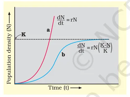
• Exponential (J-shaped): dN/dt = rN — rapid growth when resources are unlimited; r is intrinsic rate of increase.
• Logistic (S-shaped): dN/dt = rN(1 - N/K) — growth slows as population approaches carrying capacity K due to environmental resistance.

Life Tables and Survivorship

• Life table terms: lx (survivorship), qx (mortality), mx (age-specific fecundity).
• Net reproductive rate: R0 = Σ lx mx. If R0 > 1 population grows; < 1 it declines.
• Survivorship curves: Type I (low juvenile mortality, high old-age mortality), Type II (constant mortality), Type III (high juvenile mortality).

Interactions among Organisms

• Intraspecific competition: between individuals of same species (limits population size).
• Interspecific interactions: competition, predation, parasitism, mutualism (both benefit), commensalism (one benefits, other neutral), amensalism (one harmed, other neutral).
• Keystone species: species with disproportionate effect on community structure (e.g., sea otters controlling urchins).

Human Impacts: habitat destruction, pollution, overexploitation, invasive species alter environments and population dynamics; conservation aims to maintain habitats, genetic diversity and ecosystem functions.

Fig 2 — Educational Diagram: Habitat and Niche

Habitat is the physical place or environment where an organism lives — the address of the organism. It includes abiotic factors (temperature, light, soil, water, salinity) and biotic factors (food, predators, competitors) that characterize that place. Habitats can be described at different scales: macrohabitat (forest, lake, desert) and microhabitat (under a rock, leaf surface, tree canopy).

Niche is the functional role of an organism in its environment — the organism’s profession. It includes how the organism obtains resources and energy, its interactions with other species, its temporal activity (diurnal/nocturnal), and the range of environmental conditions it tolerates. Hutchinson conceptualized niche as an n-dimensional hypervolume where each axis is an environmental/resource variable.

Key distinctions:

• Habitat = place; niche = role and requirements.
• An organism can live in the same habitat as others but occupy a different niche (niche partitioning).
• Niche is multidimensional (food, temperature, nesting site, activity time), habitat is spatially defined.

Fundamental vs Realized niche:

• Fundamental niche is the full range of environmental conditions and resources an organism could theoretically use in the absence of competitors, predators or disease.
• Realized niche is the actual set of conditions and resources a species uses in nature, restricted by biotic interactions (competition, predation, parasitism).

Ecological consequences and concepts:

• Niche partitioning reduces competition and allows coexistence (e.g., different feeding zones or times).
• Competitive exclusion principle: two species with identical niches cannot stably coexist in the same habitat.
• Specialist species have narrow niches; generalists have broad niches — implications for vulnerability to environmental change.

Human relevance: understanding habitat and niche is essential for conservation (identifying critical habitat), restoration (recreating niche conditions), invasive species management (predicting potential realized niche), and predicting effects of climate change (shifts in suitable habitat and niche breadth).

Fig 3 — Educational Diagram: Adaptations to Environment

Adaptation is a heritable feature (structural, physiological or behavioural) that increases an organism's fitness in a particular environment. Adaptations arise by natural selection: individuals with traits that confer higher survival or reproductive success leave more offspring, so those traits increase in frequency.

Types of adaptations:

• Structural (Morphological): External features that help survival (e.g., thick fur, spines, leaf shape).
• Physiological (Functional): Internal biochemical or physiological processes (e.g., antifreeze proteins, CAM photosynthesis, concentration of urine).
• Behavioural: Actions or patterns of activity (e.g., migration, nocturnality, burrowing, huddling).

Key concepts:

• Trade-offs: An adaptation that benefits one function can cost another (e.g., thick fur reduces heat loss but increases heat retention in summer).
• Acclimatization vs. Adaptation: Acclimatization (phenotypic plasticity) is a reversible physiological change in an individual within its lifetime; adaptation is genetic and occurs across generations.
• Scaling and size effects: Surface area-to-volume ratio (SA:V) affects heat and water exchange; small animals lose heat faster than large ones and show different adaptations (insulation, metabolic rate).
• Ecological tolerance: Each species has a tolerance range (minimum, optimum, maximum) for environmental variables (temperature, salinity, moisture), often shown as a tolerance (performance) curve.

Examples of adaptive strategies by environment:

• Cold environments: Endothermy with insulation (fur, blubber), counter-current heat exchange in limbs, larger body size (Bergmann’s rule), compact appendages (Allen’s rule), antifreeze proteins in some fish.
• Hot/dry environments: Water storage (camels), reduced leaf area and thick cuticle in xerophytic plants, CAM and C4 photosynthesis to reduce water loss, nocturnal behaviour.
• Aquatic and saline environments: Osmoregulation (marine fish drink and excrete salts, freshwater fish excrete dilute urine), mangroves with salt-excreting glands and pneumatophores, halophyte ion compartmentalization.
• Variable environments: Diapause, migration, extreme fecundity or seed dormancy as bet-hedging strategies.

Understanding adaptations requires linking form and function, physiological mechanisms, and evolutionary processes that shape populations over time.

Fig 4 — Educational Diagram: Population — Basic Concepts

Population: A population is a group of individuals of the same species that live in a particular area at the same time and are capable of interbreeding. In ecology the term emphasizes interaction among members and with their environment.

Key attributes of a population:

• Population size (N): total number of individuals.
• Population density: number of individuals per unit area or volume (e.g., individuals km-2).
• Population distribution (dispersion): spatial arrangement of individuals — clumped, uniform (regular), or random.
• Age structure: proportion of individuals in different age classes; often shown as an age pyramid for humans or cohorts for animals.
• Sex ratio: proportion of males to females; affects reproductive potential.
• Natality and mortality: birth rate (natality) and death rate (mortality) determine changes in N.
• Immigration and emigration: individuals moving into or out of a population change N.
• Growth rate: net change per unit time determined by births, deaths, immigration and emigration.

Population change — basic model: Change in population size over time can be written as
dN/dt = (B - D) + (I - E), where B = births, D = deaths, I = immigration, E = emigration. In a closed population (no migration) this simplifies to dN/dt = B - D.

Per capita rates and intrinsic rate: If b and d are per capita birth and death rates respectively, intrinsic (per capita) rate of increase r = b − d. Then for continuous growth, dN/dt = rN.

Types of growth:

• Exponential (geometric) growth — occurs when resources are unlimited. Continuous model: dN/dt = rN with solution N(t) = N0 e^{rt}. Discrete (per generation): N_{t+1} = λ N_t, where λ is finite rate of increase.
• Logistic growth — growth limited by carrying capacity. dN/dt = rN (1 − N/K), where K is carrying capacity. Produces an S-shaped (sigmoid) curve: rapid growth when N << K, slowing as N → K, and equilibrium at N = K.

Carrying capacity (K): Maximum population size that the environment can sustainably support for a species, given available resources, environmental conditions and interactions.

Limiting factors and population regulation:

• Density-dependent factors (effects increase with population density): competition for resources, disease, predation, parasitism, waste accumulation; these tend to regulate population and produce logistic dynamics.
• Density-independent factors (effects not related to density): natural disasters, temperature extremes, droughts; cause sudden population changes irrespective of N.

Population fluctuations and dynamics: Populations may be stable, cyclic (predator-prey oscillations like lynx and hare), irregular (boom-and-bust in insects), or show long-term trends (growth or decline). Human populations often show demographic transition (changes from high birth/death rates to low birth/death rates) and specific age-structure patterns.

Sampling and estimation methods (to measure N and density): quadrat sampling for plants and sedentary animals, line transects, mark-recapture (Lincoln-Petersen index), removal sampling, direct counts for conspicuous species. Each has assumptions and error sources.

Survivorship curves: Three general types describe age-specific mortality patterns: Type I (low juvenile mortality, high old-age mortality — e.g., humans), Type II (constant mortality rate — some birds), Type III (high juvenile mortality, few survive to adulthood — many fishes, invertebrates).

Applications and importance: Understanding population concepts is essential for conservation (setting harvest limits, protected-area sizing), resource management (fisheries, forestry), epidemiology (disease spread), and human demography (planning, public health).

Note: Models are simplifications — real populations may deviate due to age structure, spatial heterogeneity, stochastic events, and complex species interactions.

Fig 5 — Educational Diagram: Population Size and Density

Population — a group of individuals of the same species occupying a particular space at a particular time.

Population size (N) — the total number of individuals of a population in a defined area or volume.

Population density (D) — the number of individuals per unit area (or unit volume). It describes how crowded a population is and is calculated as:

D = N / area (or volume)

Why measure size and density? Density affects interactions (competition, predation, disease), reproductive success, resource use and management decisions (conservation, harvesting, pest control).

Methods to estimate population size and density

• Complete enumeration (census): Counting every individual. Practical for small, accessible populations (e.g., birds in a small island, trees in a small plantation).
• Quadrat sampling: For plants or sessile animals. Place randomly located quadrats of known area, count individuals in each, compute mean density per quadrat, then extrapolate to the whole area.
• Transect sampling: Count individuals along a line (belt transect) or point counts at intervals; useful for vegetation gradients and mobile but detectable organisms.
• Mark–recapture (Lincoln–Petersen method): For mobile animals. Capture and mark n1 individuals, release them. After mixing, capture n2 individuals; m2 are marked. Estimate total population N ≈ (n1 × n2) / m2. Assumptions: closed population, marks are not lost, marked individuals mix randomly, sampling is random.
• Indirect methods: Use signs (droppings, nests, calls) or removal counts to infer density when direct counts are impractical.

Estimating from quadrats — practical steps

• Place several quadrats of known area randomly or systematically.
• Count individuals in each quadrat.
• Mean density per quadrat = (sum of counts) / (number of quadrats).
• Estimated total in study area = mean density × (total study area / quadrat area).

Factors affecting population size and density

• Demographic: births (B), deaths (D), immigration (I), emigration (E). Change in population size: ΔN = (B + I) − (D + E).
• Biotic factors: competition, predation, parasitism, disease, social behaviour.
• Abiotic factors: space, water, nutrients, temperature, habitat structure.
• Life history and reproductive rate (r), carrying capacity (K) of the habitat.

Patterns of spatial distribution — related to density and interactions:

• Clumped (aggregated): common when resources are patchy or social groups form.
• Uniform (even): from territoriality or competition.
• Random: rare; when resources are uniformly available and interactions are neutral.

Limitations and assumptions

• Sampling must be representative; small sample size increases error.
• Mark–recapture assumes closed population and no mark loss.
• Extrapolation assumes habitat homogeneity unless stratified sampling is used.

Applications — wildlife management, conservation (estimating endangered species), fisheries, pest control, forestry, epidemiology (population density affects disease spread).

Fig 6 — Educational Diagram: Dispersion Patterns

What is Dispersion?

Dispersion (or spatial distribution) describes how individuals of a species are arranged in space within a population. It is a key property of populations because it affects interactions (competition, mating, predation), sampling, and population dynamics.

Main types of dispersion

• Clumped (Aggregated): Individuals occur in groups or patches. This is the most common pattern in nature. Causes: patchy resources, social behavior, asexual reproduction, or safety in numbers.
• Uniform (Regular): Individuals are more evenly spaced than expected by chance. Causes: territoriality, competition for evenly distributed resources, allelopathy.
• Random: Individuals are spaced unpredictably, with no strong attraction or repulsion. Occurs when resources are uniformly available and interactions are neutral; often modeled by a Poisson process.

Ecological causes and significance

• Resource distribution: clustered resources → clumped individuals; evenly limiting resources → uniform spacing.
• Behaviour: social species (herds, flocks) → clumped; territorial species → uniform.
• Reproduction and dispersal mechanisms: limited dispersal (seeds falling near parent) → clumped; wind dispersal with uniform environment → random.
• Effects: Dispersion affects encounter rates (mating, predation), disease spread, and sampling accuracy (clumped populations require different sampling effort).

Measuring dispersion

Field ecologists typically sample a set of quadrats (or sampling units) and record the count (xᵢ) in each. Statistical indices compare variance to mean to infer pattern.

Interpretation

• Variance much greater than mean → clumped (aggregated).
• Variance ≈ mean → random (Poisson).
• Variance much less than mean → uniform (regular).

Notes for CBSE students

Understand the qualitative differences, be able to name real-life examples, and know simple indices used in class (variance/mean ratio). You may be asked to interpret counts from quadrats or to draw spatial patterns.

Fig 7 — Educational Diagram: Natality, Mortality and Growth Rate

Definitions: Natality (birth rate) is the production of new individuals by birth, hatching or germination in a population per unit time. Mortality (death rate) is the loss of individuals from a population by death per unit time. Population growth rate is the net change in population size per unit time resulting from births, deaths, immigration and emigration.

Measures and units: Natality and mortality are often expressed as rates per individual per unit time (per year) or as crude rates per 1,000 individuals per year. Example expressions:

• Crude birth rate = (Number of births in a time period / Average population) × 1,000
• Crude death rate = (Number of deaths in a time period / Average population) × 1,000

Per-capita (instantaneous) rates: Use small-letter notation for per-capita rates (b = per-capita birth rate, d = per-capita death rate). For a closed population (no migration): r = b − d, where r is the intrinsic (per-capita) rate of increase. If immigration (i) and emigration (e) are included: r = b − d + i − e.

Growth models:

• Geometric (discrete) growth (non-overlapping generations): Nt = N0 × λ^t, where λ (finite rate of increase) = Nt+1 / Nt. If λ > 1 population grows, λ = 1 stable, λ < 1 declines.
• Exponential (continuous) growth (overlapping generations): Nt = N0 × e^{rt}. This produces a J-shaped curve when resources are unlimited.
• Logistic growth (realistic, resource-limited): dN/dt = rN(1 − N/K), where K is carrying capacity. Solution yields an S-shaped (sigmoid) curve; growth slows as N → K.

Doubling time: Time required for a population to double under constant r: Td = ln(2) / r (for continuous growth). For geometric growth, Td = ln(2) / ln(λ).

Factors affecting natality and mortality: Internal factors—age structure, sex ratio, genetic health, physiological condition. External factors—food availability, predators, disease, climate, catastrophes. Density-dependent factors (competition, disease) change rates with population size; density-independent factors (temperature, storms) do not.

Age structure and population trajectories: Populations with many reproductive-age individuals tend to grow quickly. Age pyramids visually show a growing (wide base), stable (rectangular), or declining (narrow base) population.

Ecological significance: Natality and mortality determine population dynamics, community interactions and conservation decisions (harvesting, endangered species recovery). Understanding r and K helps predict outbreaks, collapses (overshoot and crash) and management outcomes.

Fig 8 — Educational Diagram: Age Structure and Sex Ratio

Age structure describes the distribution of individuals of different ages within a population. Ecologists usually divide a population into three age classes: pre-reproductive (young), reproductive (mature) and post-reproductive (old). Age structure is commonly shown as an age pyramid (population pyramid) with age classes on the vertical axis and number or percentage of individuals on the horizontal axis (often split by sex).

Why it matters: age structure determines a population's growth potential, future reproductive output and dependency burden. A population with a large pre-reproductive cohort tends to grow rapidly; one with many post-reproductive individuals is likely to age or decline. Age structure also affects resource use, planning for schools/healthcare and evolutionary dynamics.

Important concepts:

• Age classes/cohorts: individuals born in the same time interval form a cohort that can be followed through time.
• Population pyramid types: expansive (broad base), stationary (rectangular), and constrictive (narrow base) — each indicates different growth patterns.
• Dependency ratio: the proportion of dependents (commonly 0–14 and 65+) relative to the working-age population (15–64).

Sex ratio is the relative number of males and females in a population. In human demography (CBSE convention) sex ratio is usually expressed as the number of females per 1,000 males. There are three related measures:

• Primary sex ratio — ratio at conception (usually close to 1:1 by evolutionary theory/Fisher's principle).
• Secondary sex ratio — ratio at birth (often slightly male-biased in humans, e.g. ~950–975 females per 1000 males or about 1.05 male births per female birth depending on population).
• Tertiary sex ratio — ratio in adult or older age classes (can be female-biased because male mortality is often higher).

Causes of skewed sex ratios: differential mortality (sex-specific survival), sex-selective practices (in humans), migration (often male-biased), environmental sex determination (some reptiles), and parental allocation strategies in some animals.

Consequences: skewed sex ratios affect mating systems, reproduction rates, social structure, population viability and long-term survival. For humans, skewed sex ratios can influence marriage patterns, crime rates and social policy needs.

Sampling and presentation: Age structure and sex ratio are typically determined from census data or sample surveys and presented as histograms or pyramids split by sex. Analyses often compute proportions of each age class, median age and dependency ratios to summarize population characteristics.

Fig 9 — Educational Diagram: Survivorship Curves and Life Tables

Overview: Survivorship curves and life tables are tools used in ecology to describe how mortality and survival are distributed across ages in a population. They help compare life-history strategies, predict population growth, and understand reproductive contributions of different age classes.

Survivorship curves plot the proportion of a cohort (group of individuals born at the same time) still alive at each age (x). The vertical axis is survivorship (l_x, often the proportion surviving to age x) and the horizontal axis is age or life stage.

• Type I — low mortality in early/middle life, high mortality in old age. Curve is concave down then steep near the end. Typical of K-selected species that invest heavily in few offspring (e.g., humans, large mammals like elephants).
• Type II — roughly constant mortality rate across ages; straight line decline on a linear plot. Examples: many birds, some rodents, certain lizards.
• Type III — very high mortality early in life, survivors live relatively long. Curve drops sharply at young ages then levels off. Typical of r-selected species that produce many offspring with little care (e.g., oysters, many fishes, many plants, sea turtles where few hatchlings survive to adulthood).

Life tables (cohort or static) summarize survival and reproduction by age class. A simple cohort life table contains columns such as:

1. x — age class (0,1,2,...)
2. n_x — number alive at start of age x (raw counts)
3. l_x — survivorship = proportion surviving to age x (l_x = n_x / n_0)
4. d_x — number dying during age interval x to x+1 (d_x = n_x - n_{x+1})
5. q_x — age-specific mortality (probability of dying in interval) (q_x = d_x / n_x = 1 - p_x)
6. p_x — survival probability to next age (p_x = n_{x+1} / n_x)
7. m_x — age-specific fecundity (average number of female offspring produced by an individual of age x)

Key demographic summaries derived from a life table:

• Net reproductive rate R0 = Σ (l_x · m_x). R0 is the average number of daughters produced per female over her lifetime. If R0 > 1 the population tends to grow, R0 < 1 it tends to decline.
• Generation time G = (Σ x · l_x · m_x) / R0. G is the average age of mothers at the birth of their offspring.
• Intrinsic rate of increase r ≈ ln(R0) / G (approximate when age classes are discrete). The finite rate of increase λ = e^r ≈ R0^(1/G).

How to use these tools:

• Construct a life table from cohort counts or age-structured samples, compute l_x and m_x, then calculate R0, G and r to assess population trend.
• Plot survivorship curves (l_x vs x) to compare species or populations and infer life-history strategy (K vs r selection).
• Plot l_x·m_x vs x to see which age classes contribute most to population growth (important for conservation/harvesting management).

Notes: For continuous-time models, survivorship may be written l(x) = exp( -∫_0^x μ(t) dt ), where μ(t) is the instantaneous mortality (hazard) rate.

Fig 10 — Educational Diagram: Population Growth Models

Definition: Population growth models are mathematical descriptions of how the size of a population (N) changes with time (t) under given conditions. They simplify biological processes to explain patterns and predict trends.

Main types:

• Exponential (geometric) growth: Describes unlimited growth when resources are abundant and no density-dependent limits operate. The population increases at a rate proportional to its size, producing a J-shaped curve.
• Logistic growth: Describes growth limited by environmental carrying capacity (K). Growth slows as population approaches K, producing an S-shaped (sigmoid) curve.

Key concepts and parameters:

• N = population size at time t
• N₀ = initial population size
• r = intrinsic (per capita) rate of increase (birth rate minus death rate for continuous models)
• λ (lambda) = finite rate of increase per time step for discrete models (λ = 1 + r per generation in simple cases)
• K = carrying capacity — maximum population the environment can sustain

Exponential (continuous) model: Assumes unlimited resources and density-independent growth. The change in population is proportional to current population:

dN/dt = rN

Solution: N(t) = N₀ e^rt

Features: rapid growth, J-shaped curve; used for microbes in resource-rich culture or early phases after introduction to a new habitat.

Geometric (discrete-time) growth: For populations with discrete generations (e.g., many insects):

N_t = N₀ λ^t

Logistic model (density-dependent): Incorporates limitation by resources via carrying capacity K. The rate of increase declines linearly with N:

dN/dt = rN (1 − N/K)

Analytical solution: N(t) = K / [1 + ((K − N₀)/N₀) e^−rt]

Features: initial near-exponential phase, deceleration as resources become limiting, approach to stable equilibrium at K (stationary phase). This yields an S-shaped (sigmoid) curve.

Phases of logistic growth:

• Lag phase: slow initial growth if N₀ small or adapting
• Exponential (log) phase: rapid increase when resources abundant
• Deceleration phase: growth rate slows as density-dependent factors act
• Stationary (equilibrium) phase: N ≈ K
• Decline (sometimes): if resources fall below replacement or due to overshoot and crash

Density-independent vs density-dependent factors:

• Density-independent: affect population regardless of size (e.g., natural disasters, temperature)
• Density-dependent: change with population size and tend to regulate it (e.g., competition, disease, predation)

Assumptions and limitations: Models assume homogeneous individuals, constant r (or λ), no age structure, closed population (no migration) unless modified. Real populations may need age-structured or stochastic models.

Applications: Conservation biology (setting harvest limits), pest control, epidemiology basics, understanding human population trends, laboratory microbial growth studies.

Fig 11 — Educational Diagram: r- and K-selection Theory

Overview: r- and K-selection is a framework in life-history ecology that explains two ends of a continuum of reproductive strategies shaped by natural selection. The terms come from the variables r (intrinsic rate of increase) and K (carrying capacity) in population growth models. Species evolve traits that maximize fitness either by maximizing population growth when resources are abundant (r-selection) or by competing effectively when populations are near carrying capacity (K-selection).

r-selection (r-strategy):

• Favours high intrinsic rate of increase (high r).
• Traits: early maturity, short generation time, small body size, high fecundity (many small offspring), minimal parental care, high dispersal ability.
• Adaptive when environments are unpredictable or when vacant habitats/resources are available (density-independent mortality dominates).

K-selection (K-strategy):

• Favours traits that improve competitive ability and survival near carrying capacity K.
• Traits: late maturity, larger body size, low fecundity (few larger offspring), extensive parental care, longer lifespan.
• Adaptive in stable environments where population sizes are near resource limits (density-dependent factors important).

Life-history trade-offs: Energy and resources allocated to reproduction, growth, and survival are limited. r-selected species allocate more to reproduction; K-selected species allocate more to individual survival and competitive ability. Most real species lie along a continuum between pure r and pure K strategies.

Relation to population models: r and K appear in simple population growth equations. The exponential growth model uses r (dN/dt = rN) and describes rapid growth when resources are unlimited. The logistic growth model incorporates carrying capacity K (dN/dt = rN(1 - N/K)) and describes growth that slows as population approaches K. K-selected species tend to live near K; r-selected species show boom-and-bust dynamics described by exponential-like growth.

Limitations: The r/K framework is a simplification. Not all species fit cleanly into categories; life histories are shaped by many ecological and evolutionary factors (predation, disturbance, resource variability, social structure).

Fig 12 — Educational Diagram: Population Regulation and Limiting Factors

Overview
Population regulation refers to the ecological processes that keep population size and growth in check so that a population often remains near a characteristic level (often around the carrying capacity of the environment). Regulation arises from interactions between population intrinsic properties (birth rate, death rate, reproductive potential) and environmental factors that limit or slow growth.

Key concepts

• Biotic potential (intrinsic growth capacity): the maximum reproductive capacity of a population under ideal conditions.
• Carrying capacity (K): the maximum population size that an environment can sustain indefinitely given available resources, space, and other constraints.
• Density-dependent factors: factors whose effects change with population density. Examples: competition for resources, predation, disease, parasitism, territoriality, accumulation of wastes. These provide negative feedback: as density rises, birth rates fall and/or death rates rise.
• Density-independent factors: factors that affect population size irrespective of density. Examples: hurricanes, droughts, temperature extremes, fires. These can cause sudden population declines but do not produce regulation that depends on current population size.
• Limiting factors: any environmental attribute (nutrient, light, water, space, temperature) that constrains population growth. Liebig's law of the minimum states that growth is limited by the single scarcest resource. Shelford's law of tolerance adds that organisms have optimal and tolerance ranges for environmental factors; beyond limits, survival and reproduction decline.

Population growth models and regulation

1) Exponential growth (unlimited resources): dN/dt = rN, where N is population size and r is intrinsic rate of increase. Exponential growth gives a J-shaped curve and is typical for populations in newly available, resource-rich environments (e.g., microbes in fresh medium).

2) Logistic growth (resource-limited): dN/dt = rN(1 - N/K). The term (1 - N/K) reduces growth rate as N approaches K, producing an S-shaped (sigmoid) curve. This model captures density-dependent regulation: growth slows and stabilizes near carrying capacity.

Mechanisms of regulation (examples of density-dependent processes)

• Intraspecific competition: for food, nesting sites or mates reduces growth and fecundity as density increases.
• Predation: predator numbers may increase when prey are abundant, increasing prey mortality and causing oscillations.
• Disease and parasitism: spread more readily at high host densities, increasing mortality or reducing reproduction.
• Social stress and territoriality: crowding can reduce reproduction through stress or prevent access to breeding sites.

r- and K-selection
Species may be broadly characterized by life-history strategies: r-selected species have high reproductive rates and exploit unstable environments (e.g., many insects, bacteria); K-selected species invest more in fewer offspring, live near K, and show high competitive ability (e.g., elephants, many large mammals).

Human relevance
Understanding regulation and limiting factors is vital for conservation (managing endangered species), pest control, fisheries management (preventing overfishing that lowers K), agriculture (nutrient limits), and predicting disease outbreaks.

Fig 13 — Educational Diagram: Intraspecific and Interspecific Interactions

Overview
Intraspecific and interspecific interactions describe how organisms of the same species (intraspecific) or of different species (interspecific) affect each other's survival, reproduction and population dynamics. These interactions shape community structure, influence population size and regulate resource use.

Intraspecific interactions
These occur among individuals of the same species. Key types and consequences:

• Competition (−, −): Individuals compete for limited resources (food, mates, space). It is density-dependent—intensity increases with population density. Outcome influences carrying capacity (K) and can cause self-thinning.
• Cooperation and social behaviour (+, +): Group hunting, cooperative breeding, colony formation increase survival and reproductive success (e.g., wolf packs, eusocial insects).
• Reproductive interactions: Courtship, mate choice and sexual selection affect allele frequencies and population structure.
• Territoriality: Defence of space reduces competition for resources and breeding sites.
• Allee effect: At very low population densities, individuals may have reduced survival or reproduction (difficulty finding mates, low group defense), causing a positive correlation between density and individual fitness.

Interspecific interactions
These occur between different species. Major categories (with typical sign effects on species A, B):

• Competition (−, −): Two species vie for the same limited resource (e.g., barnacles competing for space on a rock).
• Predation (+, −): Predator benefits, prey is harmed (e.g., lion and zebra).
• Parasitism (+, −): Parasite benefits at host's expense (e.g., tapeworms in mammals).
• Mutualism (+, +): Both species benefit (e.g., pollinators and flowering plants; mycorrhizae and plant roots).
• Commensalism (+, 0): One benefits, the other is unaffected (e.g., epiphytic orchids on trees).
• Amensalism (−, 0): One is harmed, the other unaffected (e.g., penicillium secreting antibiotic that kills bacteria).
• Neutralism (0, 0): Little or no direct interaction.

Ecological and evolutionary consequences
Interactions determine resource partitioning, niche differentiation, coevolution (e.g., predator–prey arms races, host–parasite evolution), community composition, and stability. Competitive exclusion principle: two species competing for identical resources cannot stably coexist; one will exclude the other or niche differentiation will occur.

Link to population models
Intraspecific competition influences carrying capacity (K) and is included in logistic growth models. Interspecific interactions are modeled by extended equations (Lotka–Volterra) to predict dynamics like oscillations (predator–prey) or competitive outcomes.

Fig 14 — Educational Diagram: Sampling Methods and Practical Techniques

Overview: Sampling methods are procedures used to estimate abundance, density and distribution of organisms when counting every individual is impractical. Proper sampling gives representative information about populations and communities.

Key concepts:

• Density = number of individuals per unit area (or volume).
• Frequency = proportion (or %) of sampling units in which a species occurs.
• Abundance = average number of individuals per occupied sampling unit.

Sampling strategies:

• Random sampling — sampling units (e.g., quadrats) placed at random to avoid bias. Use when habitat is relatively homogeneous.
• Systematic sampling — units placed at regular intervals (grid or transect). Useful to detect gradients or patterns in distribution.
• Stratified sampling — habitat divided into strata (zones) and samples taken within each stratum. Use when habitat is heterogeneous; improves precision.

Common field techniques:

• Quadrat sampling — square or rectangular frames (e.g., 0.25 m2, 1 m2) used to count sessile or slow-moving organisms (plants, small animals). Steps: place many quadrats (random or systematic), count individuals in each, calculate mean density and extrapolate to whole area.
• Line and belt transects — a tape/rope laid across habitat. Line transect: record species touching the line (good for distribution). Belt transect: a strip of fixed width sampled along the line (good for zonation studies).
• Mark–recapture (Lincoln index) — for mobile animals. Capture a sample, mark and release (n1). After mixing, take a second sample (n2) and count marked recaptures (m). Estimate total population using N = (n1 × n2) / m. Also mention assumptions (closed population, marks not lost, random mixing, equal catchability).
• Direct counts & indirect methods — direct visual counts (birds, large mammals), or indirect signs (dung, pellets, nests, tracks) to estimate presence/abundance.

Practical tips & sources of error:

• Choose appropriate quadrat size and number: larger quadrats reduce variance for clustered organisms, more replicates increase precision.
• Avoid observer bias — standardize counting rules and training.
• Be aware of temporal variation (time of day, season) — sample repeatedly if necessary.
• Mark–recapture assumptions violations (immigration, emigration, births, deaths, trap-shyness) bias estimates.

Interpretation: Use mean densities, frequencies and abundance together to describe population structure and distribution. Use transects to detect environmental gradients (e.g., change in species composition from shore to inland) and graphs to visualise patterns.

Fig 15 — Educational Diagram: Population Dynamics and Human Population

Overview
Population dynamics is the study of how and why the number of individuals in a population changes over time and space. For organisms and populations, key processes that change population size are natality (births), mortality (deaths), immigration and emigration. Human population dynamics apply the same principles but are shaped strongly by social, economic and technological factors.

Key concepts

• Population size (N) – total number of individuals.
• Population density – number of individuals per unit area or volume.
• Dispersion pattern – clumped, uniform or random distribution of individuals.
• Age structure – proportion of individuals in different age classes; affects future growth.
• Sex ratio – male to female proportion; important for potential reproductive output.
• Life table – tabulation of age-specific survival and fecundity used to estimate population growth.
• Survivorship curves – Type I (high survival, low juvenile mortality), Type II (constant mortality), Type III (high juvenile mortality).

Population growth models

• Exponential growth (ideal conditions, unlimited resources): populations grow proportionally to current size. Characteristic J-shaped curve. Equation: dN/dt = rN, where r is intrinsic rate of increase.
• Logistic growth (limits of environment): growth slows as population approaches carrying capacity K, producing an S-shaped curve. Equation: dN/dt = rN(1 - N/K).
• Carrying capacity (K) – maximum population size the environment can sustain indefinitely.

Regulation factors

• Density-dependent factors – operate more strongly at high densities (competition, disease, predation, resource limitation).
• Density-independent factors – affect populations regardless of density (climate events, natural disasters).

Human population specifics

• Demographic parameters: crude birth rate (CBR), crude death rate (CDR), rate of natural increase (CBR - CDR), and net migration.
• Demographic transition model describes change from high birth/death rates to low birth/death rates through stages associated with industrialization and socio-economic development (classically 4 stages: pre-industrial, transitional, industrial, post-industrial; some models include a 5th stage of population decline).
• Population pyramid types: expansive (broad base, rapid growth), constrictive (narrow base, declining growth), stationary (roughly rectangular, stable).
• Contemporary issues: ageing populations in developed countries, continued rapid growth in some developing regions, urbanization, migration, resource demand, environmental impact and sustainable development concerns.

Applications and measurements
Life tables and cohort studies are used to compute survivorship, reproductive rates and to predict future population trends. Human population policy (family planning, health care, education) affects demographic rates and thus dynamics.

Takeaway
Population dynamics integrates biological rates (births, deaths, migration) with environmental limits and species life-history strategies. For humans, social and technological changes shift these rates, leading to characteristic demographic transitions and policy challenges.