Chapter 1 — National Income And Related Aggregates

Fig 1 — Educational Diagram: Introduction and Basic Concepts

What is National Income?
National income is the total money value of all final goods and services produced by the factors of production owned by the residents of a country during a particular period (usually a year). It is a flow variable (measured over time) not a stock.

Key aggregate concepts

• Gross Domestic Product (GDP) – Value of final goods and services produced within the domestic territory in a period (at market prices).
• Gross National Product (GNP) / GNI – GDP plus net factor income from abroad (NFIA). NFIA = factor incomes received from abroad by residents − factor incomes paid to non‑residents.
• Net Domestic Product (NDP) – GDP minus depreciation (consumption of fixed capital).
• Net National Product (NNP) – GNP minus depreciation.
• National Income (NI) / NNP at factor cost – NNP adjusted from market prices to factor cost (i.e., NNPmp − indirect taxes + subsidies). This measures incomes accruing to factors of production.
• Per capita income – National income divided by population; indicates average income per person.

Market price vs Factor cost
Market price includes indirect taxes (GST, excise) and excludes subsidies. Factor cost is the income earned by factors of production (wages, rent, interest, profit) and equals market price minus net indirect taxes (indirect taxes − subsidies).

Other important distinctions

• Nominal (current) vs Real (constant) values – Nominal GDP is valued at current year prices. Real GDP is valued at base‑year prices and removes price (inflation) effects.
• Stock vs Flow – National income is a flow (measured per year). Capital or money saved is a stock (measured at a point in time).
• Final goods vs Intermediate goods – To avoid double counting, only final goods/services are included in GDP; value added method sums value added at each stage.
• Transfer payments (pensions, unemployment benefits, remittances sent abroad) are not payments for current production and therefore are excluded from national income.

Methods of measuring national income

• Production (Output) method – Sum of value added across all producing units (firms, sectors).
• Income method – Sum of incomes earned by factors of production: wages + rent + interest + profits + mixed incomes.
• Expenditure method – Sum of final expenditures: Consumption (C) + Investment (I) + Government spending (G) + Net exports (X − M).

Uses and limitations
National income statistics are used to assess economic performance, compare living standards, guide policy. Limitations: excludes non‑market activities, informal economy, environmental degradation, distributional aspects, and may have measurement errors.

Fig 2 — Educational Diagram: Income Concepts related to Households

Overview
In the study of national income, households are the ultimate recipients of income generated in the economy. Several distinct income concepts describe how income flows from production to households and how much they can spend or save.

Key household-related income aggregates

• Private Income (PrI): Income received by the private sector (households plus private firms) before personal taxes and after adjusting for corporate items. It is obtained from National Income by subtracting certain corporate items and employers' social contributions.
• Personal Income (PI): The total income actually received by households. It equals private income plus transfer payments (government benefits, pensions, subsidies) that households receive. PI excludes corporate retained earnings and corporate taxes.
• Personal Disposable Income (PDI) (also called Disposable Income): The income households have available for spending or saving after paying personal (direct) taxes. PDI = Personal Income − Personal Taxes. This is the most important concept for analyzing consumption and saving behaviour.

Why these distinctions matter
Not all income earned in the economy reaches households. Firms retain profits or pay corporate taxes; governments redistribute part of income back to households as transfer payments. Distinguishing these aggregates helps measure households’ effective purchasing power and saving capacity.

Relationships (verbal)

1. Start with National Income (NI) — the total factor income earned by residents.
2. Subtract corporate taxes, undistributed corporate profits (retained earnings) and employers' social security contributions to get Private Income.
3. Add transfer payments (social benefits, pensions, unemployment allowances) to Private Income to obtain Personal Income.
4. Subtract personal taxes (income tax, property tax paid by households) from Personal Income to get Personal Disposable Income.

Consumption and saving
Personal Disposable Income is split between consumption (C) and personal saving (S): PDI = C + S. Thus, PDI determines household demand and saving behaviour.

Fig 3 — Educational Diagram: Net Factor Income from Abroad (NFIA) and Net Domestic/Foreign Distinctions

Definition — NFIA
Net Factor Income from Abroad (NFIA) is the difference between factor incomes (wages, rent, interest, profit) received by residents of a country from the rest of the world and factor incomes paid by residents to the rest of the world:

NFIA = Factor income received from abroad − Factor income paid to abroad

Why NFIA matters
NFIA converts a measure that is location-based (GDP: output produced within a country’s territory) into a residence-based measure (GNP/GNI: income of a country's residents). If NFIA is positive, residents earn more from abroad than they pay out — so GNP > GDP. If NFIA is negative, GNP < GDP.

Domestic vs Resident (National) Distinction

• Domestic territory (location concept): economic activities performed within the geographic boundaries of a country, irrespective of who performs them. GDP (Gross Domestic Product) measures value of production within this territory.
• Residents (nationality/center of economic interest) (residence concept): persons/units whose center of economic interest is in the country for a specified period (usually one year), regardless of where production takes place. GNP/GNI measures income accruing to these residents.

How NFIA links GDP and GNP/GNI

• GDP (location-based) measures output produced domestically.
• Add NFIA (net income flows between residents and non-residents) to convert GDP into GNP/GNI (residence-based).

Practical interpretation

• If many nationals work abroad and send remittances, NFIA tends to be positive.
• If many foreign firms earn and repatriate profits from domestic production, NFIA tends to be negative.

Accounting chain (typical relations)

• GDP at market prices (GDPmp)
• GDP at factor cost (GDPfc) = GDPmp − Indirect taxes + Subsidies
• GNP at market prices (GNPmp) = GDPmp + NFIA
• GNP at factor cost (GNPfc) = GNPmp − Indirect taxes + Subsidies
• NNP (Net National Product) at factor cost (NNPfc) = GNPfc − Depreciation

Key points to remember

• NFIA is about factor income flows (wages, interest, dividends, rent, profits), not goods and services trade (that is NX/BoP current account items related but distinct).
• GDP and GNP differ only by the net factor income from abroad.
• Resident vs domestic distinction is central for compiling national accounts and for policy interpretation (employment abroad, capital flows, external dependence).

Fig 4 — Educational Diagram: Methods of Measuring National Income

Overview
National income is the total money value of final goods and services produced by an economy in a year. There are three standard methods to measure national income (they should, in principle, give the same result): the Product (Value‑Added) method, the Income method, and the Expenditure method. Each method requires specific adjustments (depreciation, indirect taxes and subsidies, net factor income from abroad) to convert gross/domestic measures into the commonly used national income concept (typically NNP at factor cost).

1. Product (Output / Value‑Added) Method

• Idea: Sum the value of final goods and services produced OR sum value added at each production stage across all firms and industries.
• Value added at a firm = Value of output produced − Value of intermediate consumption (inputs purchased from other firms). This avoids double counting.
• Steps: calculate gross value added (GVA) for each sector (agriculture, industry, services), sum them to get total GVA. Then adjust product taxes and subsidies to get GDP at market prices.
  • GVA (basic prices) + Taxes on products − Subsidies on products = GDP at market prices (GDPmp).
• Practical tip: Break the economy into sectors and sum each sector's GVA (or use final goods’ market values when available).

2. Income Method

• Idea: Sum incomes earned by factors of production in the economy: wages and salaries, rent, interest, profits and mixed income (self‑employed).
• Steps: Add up all factor payments (compensation of employees + rent + interest + profits + mixed income). If you want national income rather than domestic product, add Net Factor Income from Abroad (NFIA). To go from market prices to factor cost, subtract indirect taxes and add subsidies.
• Result: This gives national income at factor cost (after required adjustments becomes NNP at factor cost).

3. Expenditure Method

• Idea: Sum total expenditure on final goods and services in the economy by all sectors: households, firms, government and foreign sector.
• Formula: GDP at market prices = C + I + G + (X − M), where
• C = Private final consumption expenditure (household consumption)
• I = Gross domestic capital formation (investment: business fixed investment + inventories + residential)
• G = Government final consumption expenditure
• X = Exports of goods and services
• M = Imports of goods and services (subtracted)
• After computing GDP (expenditure), make adjustments (depreciation, NFIA, indirect taxes/subsidies) to reach the desired national income concept.

Important adjustments and relationships (how to move between measures)

• From domestic to national: add Net Factor Income from Abroad (NFIA = factor income received from abroad − factor payments to abroad).
• Gross ↔ Net: Subtract depreciation (consumption of fixed capital) to go from gross to net.
• Market prices ↔ Factor cost: Subtract indirect taxes and add subsidies to go from market prices to factor cost.

Common problems / limitations

• Non‑market (household) production and unpaid work are not valued; understate real output.
• Underground economy and tax evasion lead to underestimation.
• Double counting if intermediate goods are included in final totals (avoided by value‑added approach).
• Price changes (inflation) distort comparisons over time unless data are converted to real terms (deflation using price indices).
• Data collection difficulties, timing lags and valuation at current prices vs constant prices.

How CBSE/NCERT typically present the flow: In exams you'll be asked to describe the three methods, write the key formula for the expenditure approach, explain value‑added calculation with a simple example, list components of factor income, and note important adjustments (depreciation, indirect taxes, subsidies, NFIA) and limitations.

Fig 5 — Educational Diagram: Value Added and Avoidance of Double Counting

What is Value Added?

Value added at a production stage is the additional value created by a firm or activity. Formally: Value added = Value of output − Value of intermediate consumption. Intermediate consumption means goods and services used up in producing the output during the accounting period.

Why double counting happens

• Double counting occurs when we add the value of intermediate goods to the value of final goods. If the same good is counted at each stage of production as part of output, the total will exceed the value of final products and overstate national income.
• Example of double counting: if a farmer's sale of wheat, a miller's sale of flour and a baker's sale of bread are all summed as output, the wheat and flour are counted more than once.

How double counting is avoided

There are two standard methods used in national accounts to avoid double counting:

1. Final goods and services method: Count only the value of final goods and services produced within the period (goods sold for final consumption or investment). Intermediate goods transactions are excluded.
2. Value added method (recommended): Compute value added at each production stage (output minus intermediate consumption) and sum the value added for all firms/activities. The sum of value added equals the value of final output.

Relation to GDP and related aggregates

When summed across all firms, value added gives Gross Value Added (GVA). Adjusting GVA for taxes and subsidies on products converts it to GDP at market prices. Subtracting depreciation yields Net Domestic Product (NDP).

Key conceptual points:

• Only final goods and services or value added should be counted to measure national income accurately.
• Used goods, pure financial transfers (like pensions, gifts), and second-hand sales are excluded from GDP (they do not represent current production).

Fig 6 — Educational Diagram: Real vs Nominal Measures and Price Indices

Overview

In national accounts and everyday economics we distinguish between nominal and real measures. A nominal measure is expressed in current money prices of the time when the quantity was produced or measured. A real measure is adjusted for changes in the price level (inflation or deflation) so it shows the quantity in terms of constant purchasing power (a base year). Price indices are statistical tools that measure the average change in prices over time and are used to convert nominal values into real values.

Nominal vs Real — key ideas

• Nominal value: Measured in current prices. Example: Nominal GDP in 2024 is the value of all goods and services produced in 2024 at 2024 prices.
• Real value: Measured in constant (base year) prices. Example: Real GDP in 2024 is the value of 2024 production valued at base-year prices; it shows quantity changes only.
• Real values remove the effect of price changes, so they allow comparison of actual physical output or purchasing power across years.

Price indices — purpose and common types

• Price index: (Index number) is a relative measure showing how prices in a given year compare to prices in a base year. It is usually set to 100 in the base year.
• CPI (Consumer Price Index): Measures average price changes of a fixed basket of goods and services consumed by urban households (used to measure cost of living and inflation for consumers).
• WPI (Wholesale Price Index): Measures price changes at the wholesale / producer level (earlier used in India for inflation measurement).
• GDP deflator (Implicit Price Deflator): Broad price index for all goods and services included in GDP. It is not based on a fixed basket — weights change with the composition of output.

How indices convert nominal into real

To get a real measure from a nominal measure we divide by an appropriate price index (expressed in index form) and multiply by 100 (if index base = 100):

Real value = (Nominal value / Price Index) × 100

This removes the effect of price level changes and leaves changes due to quantities or volumes.

Types of index formulae (brief)

• Laspeyres index (base-weighted): Uses base-year quantities as weights — tends to overstate cost of living when relative prices change (substitution bias).
• Paasche index (current-weighted): Uses current-year quantities as weights — tends to understate cost of living change compared to Laspeyres.
• Fisher ideal index: Geometric mean of Laspeyres and Paasche — commonly used as a compromise.

Limitations and practical issues

• Choice of base year matters; statistical agencies periodically rebase indices.
• Fixed baskets cause substitution bias when consumers change buying patterns as prices change.
• Quality changes and introduction of new goods complicate measurement.

Fig 7 — Educational Diagram: Per Capita Income and Growth Rates

Per Capita Income (PCI)

Per capita income is an average measure of income per person in an economy. It is obtained by dividing the national income (or GDP/GNP) by the total population. PCI is used to compare living standards across time or across countries, but it is only an average and does not show distributional differences.

Why it matters

• Indicator of average material well-being and standard of living.
• Useful for cross-country comparisons (often adjusted for purchasing power parity, PPP) and for tracking welfare changes over time.

Nominal versus Real PCI

Nominal PCI is calculated using current prices. Real PCI adjusts for inflation (using a price index) and therefore shows changes in the quantity of goods and services available per person.

Growth Rates of Per Capita Income

The growth rate of per capita income tells us how fast average income per person is rising (or falling) over time. Growth in PCI depends on two factors: growth of national income and growth of population. If income grows faster than population, PCI rises; if population grows faster than income, PCI falls.

Exact relationship (using levels)

If PCI_t = NI_t / Pop_t, the exact growth rate of PCI from period t-1 to t is:

g_PCI = (PCI_t / PCI_{t-1}) - 1 = ((NI_t / Pop_t) / (NI_{t-1} / Pop_{t-1})) - 1

This can be rearranged using growth factors. In terms of percentage growth rates (g_NI for national income, g_Pop for population):

1 + g_PCI = (1 + g_NI) / (1 + g_Pop)

So the exact percentage growth is g_PCI = (1 + g_NI) / (1 + g_Pop) - 1.

Approximate relation

When growth rates are small, a good approximation is:

g_PCI ≈ g_NI - g_Pop

This is commonly used for quick estimates: the per capita growth roughly equals the difference between national income growth and population growth.

Limitations of PCI

• Does not reflect income distribution or inequality.
• May hide regional differences and informal/unreported incomes.
• Nominal PCI can be misleading if inflation is high — always prefer real PCI for temporal comparisons.

Practical points for CBSE students

• Always state whether PCI is based on GDP, GNP, or national income and whether it is nominal or real.
• When asked to compute growth rates, show the formula and clearly indicate periods.
• When comparing countries, mention PPP adjustment if price level differences matter.

Fig 8 — Educational Diagram: Circular Flow of Income

What it is: The circular flow of income is a basic macroeconomic model that shows how money, goods and services, and factors of production move between different sectors of the economy. It explains how total income (national income) is generated and distributed, and how spending and earning are linked.

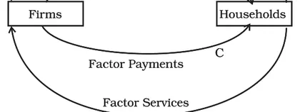
Key idea: Incomes paid to households for providing factors of production (wages, rent, interest, profit) are used to buy goods and services from firms. That spending becomes firms' revenue, which is paid back to households as income. This continuous flow creates the economy’s aggregate income and expenditure.

Models:

• Two‑sector model (Households and Firms, closed economy without government): Households supply factors to firms and receive factor payments (income). They spend on consumption (C). Firms produce output and receive consumption expenditure. Part of households' income may be saved (S) and part spent. Equilibrium requires that planned saving equals planned investment (S = I).
• Three‑sector model (adds Government): Government collects taxes (T) and injects spending (G). Taxes are a leakage; government purchases are an injection. For equilibrium: leakages (S + T) = injections (I + G).
• Four‑sector model (adds Foreign sector): Exports (X) are injections and imports (M) are leakages. The equilibrium condition becomes: S + T + M = I + G + X. In aggregate demand terms, national product/output (Y) = C + I + G + (X − M).

Leakages and injections: Leakages withdraw spending from the income flow (saving S, taxes T, imports M). Injections add spending to the flow (investment I, government spending G, exports X). For the economy to be in equilibrium, total leakages must equal total injections.

Role of financial sector: Financial institutions channel household savings into investment. Banks transform S into I through lending; this is the mechanism linking leakages to injections.

Assumptions (simple models): No price changes, no idle resources (full employment often assumed in basic circular flow), planned spending equals actual spending, sector behaviour aggregated.

Importance: The circular flow model clarifies how changes in any sector (e.g., a rise in taxes, a fall in exports, or an increase in investment) affect aggregate income, and it underpins identities used in national income accounting.

Fig 9 — Educational Diagram: Aggregate Expenditure Components

Definition: Aggregate expenditure (AE) is the total planned spending on final goods and services in an economy at a given level of national income (output). In a simple income–expenditure framework AE = C + I + G + (X - M).

Main components:

• Consumption (C): Spending by households on goods and services. It depends on disposable income (Yd = Y - T) and can be expressed by a consumption function: C = C0 + MPC × Yd, where C0 is autonomous consumption and MPC (marginal propensity to consume) is the slope.
• Investment (I): Spending by firms on capital goods, residential buildings, and changes in inventories. Investment has two parts: autonomous investment (independent of current income) and induced investment (varies with output or interest rates). Planned investment is a key determinant of equilibrium output.
• Government expenditure (G): Government purchases of goods and services. Transfer payments are not direct government purchases but affect disposable income and thus consumption.
• Net exports (X - M): Exports (X) minus imports (M). Exports are autonomous with respect to domestic income (depend on foreign demand), while imports typically rise with domestic income (M = M0 + m × Y, where m is marginal propensity to import).

Autonomous vs induced: Autonomous components (C0, autonomous I, autonomous G, autonomous X) do not depend on current income. Induced components (the portion of C and M) change with income. Aggregate expenditure as a function of income can be written AE(Y) = C0 + MPC×(Y - T) + I0 + G + X0 - M0 - m×Y.

Equilibrium condition: The goods market is in equilibrium when planned aggregate expenditure equals actual output/income: Y = AE(Y). If AE > Y, inventories fall and firms increase production (Y rises); if AE < Y, inventories rise and production falls.

Multiplier effect: A change in an autonomous component (ΔA) leads to a multiplied change in equilibrium income: ΔY = k × ΔA. In a simple closed economy without taxes and imports, k = 1/(1 - MPC) = 1/MPS. In a more realistic model with taxes (t) and marginal propensity to import (m or MPM), the multiplier is k = 1 / [1 - MPC(1 - t) + m].

Key implications: Consumption is the largest component of aggregate expenditure in most economies, so changes in income, taxes, or consumer confidence strongly affect AE. Investment is volatile and sensitive to interest rates and expectations. Government spending and net exports are important policy levers for stabilising output.

Fig 10 — Educational Diagram: Statistical Discrepancy and National Accounts Identities

What the topic covers
This topic explains the key national accounts identities (production, income and expenditure approaches to measuring national income) and why, in practice, estimates from different approaches do not match exactly — the difference is called the statistical discrepancy.

Three standard approaches to measure national income

• Production (output) approach: GDP (at market prices) = Sum of Gross Value Added (GVA) of all sectors + (taxes on products − subsidies on products).
• Income approach: GDP at factor cost = Sum of factor incomes: wages + rent + interest + profits + mixed income of self-employed.
• Expenditure approach: GDP at market prices = C + I + G + (X − M), where C = consumption, I = investment, G = government spending, X = exports, M = imports.

Key relationships / conversions

• Market price versus factor cost:
  GDP(mp) = GDP(fc) + (Indirect taxes − Subsidies). (mp = market prices, fc = factor cost)
• Gross and net:
  NDP = GDP − Depreciation (consumption of fixed capital).
• Domestic and national:
  GNP = GDP + Net Factor Income from Abroad (NFIA) (NFIA = factor income received from abroad − factor income paid abroad).
• Net national:
  NNP = GNP − Depreciation.

Where statistical discrepancy comes from
In an ideal accounting system the three approaches give the same number. In reality, they differ because of measurement and timing issues, incomplete coverage and data sources. The gap between two (or the balanced average of) estimates is recorded as the statistical discrepancy so that the accounts balance.

Typical causes

• Different data sources and surveys for income, production and expenditure (sampling and non-sampling errors).
• Timing differences (income recorded when earned vs expenditure when spent).
• Informal and unreported activity (tax evasion, household production).
• Valuation differences (market prices vs factor cost), and incorrect estimates of depreciation.
• Differences in coverage (population, sectors) or classification errors.

How statistical discrepancy is shown
National statistical offices usually present all three estimates. If they differ, a statistical discrepancy item is shown (often under the income side) so that the expenditure total equals the income total. The discrepancy is treated as an accounting balancing item, not an economic variable.

Interpretation and importance
A small discrepancy (as a percent of GDP) indicates consistent measurement; a large or growing discrepancy signals data problems and may prompt revisions to data sources, methods or benchmarking to censuses. Analysts should check trends in the discrepancy to judge the reliability of national accounts.

Fig 11 — Educational Diagram: Difficulties in Measurement

Context: Measurement of national income (GDP, GNP, NNP, national income) attempts to aggregate the monetary value of production and incomes in an economy. In practice several conceptual and practical problems make accurate measurement difficult.

Main difficulties

• Unreported / informal / underground economy: Many activities (household production, casual labour paid in cash, barter, small-scale vendors, black‑market transactions and illegal activities) are not recorded in official statistics, causing underestimation.
• Non‑market transactions: Services provided within households (cooking, childcare), volunteer work, and subsistence farming produce value but have no market price, so they are excluded or must be imputed.
• Intermediate vs final goods — double counting: If we add values of all goods produced without careful treatment, intermediate goods will be counted multiple times. National income requires counting only final goods or using value‑added methods.
• Valuation problems: Choosing market prices, imputing rents (owner‑occupied housing), and valuing barter transactions are hard. Price changes (inflation/deflation) complicate comparisons over time unless converted to constant prices.
• Quality change and new goods: Improvements in quality (e.g., smartphones) and arrival of new products deliver more real value that is hard to capture with simple price indices.
• Depreciation and capital consumption: Measuring capital consumption (wear and tear) precisely is difficult; omitting or mis‑estimating depreciation distorts net aggregates (NNP, national income).
• Transfer payments and used goods: Transfer payments (pensions, welfare) are not production and must be excluded. Trade in used goods transfers ownership but not current production and should be excluded, yet often causes confusion.
• Cross‑border factor income and statistical discrepancies: Net factor income from abroad must be added/subtracted to move between GDP and GNP. Data on remittances and factor payments can be delayed or inaccurate.
• Timeliness, coverage and collection errors: Surveys, tax records and administrative data can be incomplete, lagged, or suffer sampling/non‑sampling errors and deliberate misreporting.
• Base year and indexation problems: Choosing an inappropriate base year for constant price estimates or long gaps between base revisions produce biased real growth rates.
• Aggregation and distribution issues: National totals conceal distributional changes: rising GDP can coexist with increasing inequality or worsening welfare for many.

Method‑specific measurement issues

• Production approach: Hard to measure output in informal sectors and to estimate value added for services without clear market prices.
• Income approach: Some incomes are hidden or not declared (tax evasion), and imputations (e.g., owner occupation) are required.
• Expenditure approach: Final consumption may be underestimated (household own‑consumption), and investment estimates can miss informal investment in dwelling improvements or livestock.

Effects on indicators: These difficulties cause under/over‑estimation of national income, distort time‑series growth rates, bias international comparisons (unless PPP adjustments and consistent methods are used) and mislead policy if not corrected.

Mitigation and official practice: Statistical offices use surveys, satellite accounts (for households, informal economy), imputations (owner‑occupied rent), periodic base year updates, hedonic price adjustments for quality change, and PPP methods for international comparisons — but residual errors remain.

Conclusion: Measurement of national income gives a useful but imperfect picture. Awareness of these difficulties helps interpretation—GDP is a key indicator but not a complete measure of well‑being.

Fig 12 — Educational Diagram: Uses and Importance of National Income Statistics

National income statistics measure the total value of goods and services produced in an economy and related aggregates (GDP, GNP, NNP, per capita income, etc.). They are vital tools for understanding economic performance, planning policy, and making comparisons over time and across countries.

• Assessing economic performance and growth — Real GDP and growth rates show whether an economy is expanding or contracting and help judge the success of economic policies.
• Formulating macroeconomic policy — Governments and central banks use national income data to set fiscal policy (taxes, spending, deficit targets as a % of GDP) and monetary policy (interest rates, liquidity) according to the output gap and inflationary pressures.
• Planning and resource allocation — For national and regional planning (e.g., allocating funds across states, sectors, or programmes), national income figures show which sectors need investment or support.
• Estimating standard of living — Per capita income (national income divided by population) is a basic indicator of average living standards and is used to classify countries (low-, middle-, high-income).
• Income distribution and social policy — Combined with distributional data, national income helps design welfare policies, minimum wages, and poverty alleviation programmes (e.g., targeting subsidies or employment schemes).
• Comparisons over time and across countries — Real GDP and GDP per capita (often adjusted for purchasing power parity) allow international comparisons and trend analysis.
• Sectoral analysis and structural change — Breakdowns by agriculture, industry and services show structural transformation and guide sector-specific policies and training programmes.
• Business and investment decisions — Firms and investors use GDP trends, sectoral shares and income statistics to forecast demand, decide locations and scale of investments.
• Monitoring business cycles and crises — Quarterly/annual national income data reveal recessions, recoveries and the severity of shocks (e.g., GDP contraction during the COVID-19 pandemic), guiding relief measures.
• International obligations and finance — Donors, international organizations and rating agencies use national income measures to decide aid, loans and credit ratings.

Important caveat: While indispensable, national income figures have limitations (non-market activities, informal sector measurement problems, income distribution not shown by aggregate averages). These should be borne in mind when using the statistics for policy.

Fig 13 — Educational Diagram: Limitations of National Income as Welfare Measure

Introduction: National income (GDP/GNP/NNP) measures the market value of final goods and services produced in a period. Though useful for macroeconomic analysis, it is an imperfect indicator of social welfare. The following are the main limitations with brief explanations.

1. Does not account for distribution of income

   Aggregate national income can rise while most people do not benefit if income accrues to a small rich segment. Thus higher national income does not imply greater welfare for the majority.

2. Ignores non-market and household services

   Unpaid household work (childcare, eldercare, home production), volunteer services and subsistence farming are omitted because they do not involve market transactions, understating true welfare—especially in developing countries and for women.

3. Does not deduct negative externalities

   Economic activities that increase income (industrial output, resource extraction) can create pollution, health hazards and environmental degradation. National income typically records the gross value but not the environmental costs, so welfare may fall despite rising income.

4. Includes some activities that may reduce welfare

   Expenditures on crime control, pollution cleanup, and reconstruction after disasters raise measured national income but reflect restorative or defensive spending rather than welfare improvements.

5. Underground economy and measurement problems

   Black market transactions, tax evasion and informal economic activity are often unrecorded; hence national income may under- or mis-report actual economic activity and welfare.

6. Quality changes and new goods are hard to measure

   GDP uses prices to value output. Improvements in quality (better healthcare, technology) or the introduction of new goods/services are difficult to price accurately, leading to mismeasurement of welfare gains.

7. Population size and per capita differences

   Total national income ignores population. A large GDP with a huge population may mean low per capita income and low living standards. Per capita measures are better but still imperfect.

8. Excludes important non-economic aspects of welfare

   Factors such as health, education, life expectancy, leisure, political freedom, security and social cohesion are important to welfare but are not captured in national income figures.

9. Price level changes / inflation and comparability over time

   Nominal national income can increase due to inflation rather than real growth. Real measures exist but depend on appropriate deflators; international comparisons require PPP adjustments.

10. Treatment of transfer payments and depreciation

    Transfer payments (social security, subsidies) are not payments for current production and are excluded; depreciation reduces net measures—both affect how well national income reflects welfare.

Conclusion and alternatives: Because national income alone misses distributional, environmental and non-market dimensions of well-being, complementary indicators are used to assess welfare: per capita real income, Human Development Index (HDI), Genuine Progress Indicator (GPI), measures of income inequality (Gini coefficient), and environmental-adjusted accounts.

Fig 14 — Educational Diagram: Adjustments and Related Concepts

What the adjustments are for
When we measure national output and income we start with values observed in the market (market prices) and then make adjustments to remove distortions so that we end up with measures that reflect actual income earned by factors of production (factor cost) or the income available to households. These adjustments explain how to move between GDP, GNP, NNP, National Income, Personal Income and Personal Disposable Income.

Key concepts explained

• Final vs intermediate goods: Only final goods and services are included in GDP to avoid double counting. Intermediate goods (used up in production) are excluded.
• Transfer payments: Payments like pensions, scholarships or unemployment benefits are not payments for current production and are excluded from GDP.
• Depreciation (Consumption of fixed capital): Part of gross output that compensates for wear and tear of fixed capital. Subtract depreciation from gross product to get net product.
• Indirect taxes and subsidies: GDP at market price includes indirect taxes (e.g., GST, excise) and excludes subsidies. To convert to factor cost, subtract net indirect taxes (indirect taxes − subsidies).
• Net Factor Income from Abroad (NFIA): Income earned by a country’s residents from abroad minus income paid to foreigners. Add NFIA to domestic production to get national product (GNP).
• Statistical discrepancy: Differences that arise because income and expenditure methods of estimating national income use different data sources—recorded as balancing item if needed.
• National versus personal measures: National Income (NI) measures income earned by factors of production (NNP at factor cost). Personal Income (PI) is NI adjusted for items not received by households (corporate taxes, undistributed profits, social security contributions) and items received but not earned (transfer payments). Personal Disposable Income (PDI) = PI − personal taxes; it's income available for consumption and saving.

How the sequence of adjustments typically runs

Start: GDP (Gross Domestic Product) at market price → remove net indirect taxes → get GDP at factor cost → add NFIA → GNP at factor cost → subtract depreciation → NNP at factor cost = National Income (NI). From NI make further adjustments to get Personal Income (PI) and Personal Disposable Income (PDI).

Why these adjustments matter
They ensure that the aggregates measure what they are intended to: production within the domestic territory (GDP) versus income of residents (GNP), gross versus net (gross includes replacement of capital), and the amount actually available to households to spend or save (PDI).