Chapter 2 — Polynomials

What is a polynomial?
A polynomial in one variable x is an expression of the form a_n x^n + a_{n-1} x^{n-1} + ... + a_1 x + a_0, where each a_i is a constant (called a coefficient), n is a non‑negative integer, and a_n ≠ 0. The highest power n with a_n ≠ 0 is called the degree of the polynomial.

Parts of a polynomial
- Term: each a_i x^i is a term.
- Coefficient: the number a_i multiplying x^i.
- Constant term: a_0 (term with x^0).

Types by number of terms
- Monomial: one term (e.g. 5x^3).
- Binomial: two terms (e.g. x^2 + 3x).
- Trinomial: three terms (e.g. x^2 + x + 1).

Special polynomials by degree
- Constant polynomial: degree 0 (e.g. 7).
- Linear polynomial: degree 1 (e.g. 2x − 3).
- Quadratic polynomial: degree 2 (e.g. x^2 − 4x + 4).
- Cubic: degree 3, etc. The zero polynomial (0) has all coefficients 0; its degree is usually left undefined (or sometimes taken as −∞).

Valid vs. invalid expressions
Valid polynomials have nonnegative integer exponents and a finite number of terms. Examples that are NOT polynomials: x^{−1} (negative exponent), 1/x (variable in denominator), x^{1/2} (fractional exponent), and infinite series like 1 + x + x^2 + ⋯.

Key properties (short)
- A polynomial of degree n can have at most n distinct real zeros (roots).
- Remainder theorem: when a polynomial p(x) is divided by (x − a), the remainder is p(a).
- Factor theorem: (x − a) is a factor of p(x) iff p(a) = 0.

How polynomials appear in problems
Polynomials model many algebraic quantities: lengths, areas, volumes, cost or revenue models (linear or quadratic), and approximate curves in physics/engineering.

What is a polynomial? A polynomial in one variable x is an expression of the form a_n x^n + a_{n-1} x^{n-1} + ... + a_1 x + a_0, where each a_i is a real number (coefficient) and n is a non‑negative integer.

Degree of a polynomial
The degree of a nonzero polynomial is the highest power (exponent) of x that has a nonzero coefficient. If p(x)=a_n x^n+...+a_0 with a_n ≠ 0, then deg p(x)=n.

Leading coefficient
The coefficient a_n of the highest-power term a_n x^n is called the leading coefficient of the polynomial.

Special case — zero polynomial
The zero polynomial 0 has every coefficient equal to 0. Its degree is undefined (often treated as −∞ for algebraic convenience) and it has no well-defined leading coefficient.

How to find degree and leading coefficient — steps

• Combine like terms first (add coefficients of same power).
• Identify the term with the highest exponent whose coefficient is not zero.
• The exponent of that term is the degree; its coefficient is the leading coefficient.

Key properties

• If deg P = m and deg Q = n then deg(P+Q) ≤ max(m,n). (If leading terms cancel, the degree may be smaller.)
• If deg P = m and deg Q = n then deg(P·Q) = m + n, provided the product is not the zero polynomial.
• The leading coefficient of P·Q is the product of the leading coefficients of P and Q.
• An nth-degree polynomial can have at most n real turning points and at most n real roots (counting multiplicity).

Why it matters
Degree and leading coefficient determine the polynomial's end behavior and overall shape: for large |x| the highest-degree term a_n x^n dominates. If n is even, both ends of the graph go in the same direction; if odd, ends go in opposite directions. The sign of a_n (leading coefficient) decides whether ends go up or down.

Example (brief)
For p(x)=4x^3 - x + 7: degree = 3, leading coefficient = 4. For q(x)=x^2 - 5x + 6: degree = 2, leading coefficient = 1.

Class 10 tip: Always combine like terms before deciding degree. If leading terms cancel when adding polynomials, re-evaluate the highest remaining power.

What is a polynomial? A polynomial in one variable x is an expression of the form a_n x^n + a_{n-1} x^{n-1} + ... + a_1 x + a_0, where a_n, ..., a_0 are real numbers and n is a non-negative integer. The highest power n with a_n ≠ 0 is called the degree of the polynomial and a_n is the leading coefficient.

Classification by number of terms

• Monomial: A polynomial with one term (e.g. 5x^3, 7).
• Binomial: Two terms (e.g. x^2 + 3x).
• Trinomial: Three terms (e.g. x^2 + 5x + 6).
• Polynomial (general): More than three terms (e.g. x^4 - 2x^3 + x - 5).

Classification by degree

• Constant polynomial: Degree 0, e.g. 7.
• Linear polynomial: Degree 1, e.g. 2x + 3. Graph is a straight line.
• Quadratic polynomial: Degree 2, e.g. ax^2 + bx + c. Graph is a parabola.
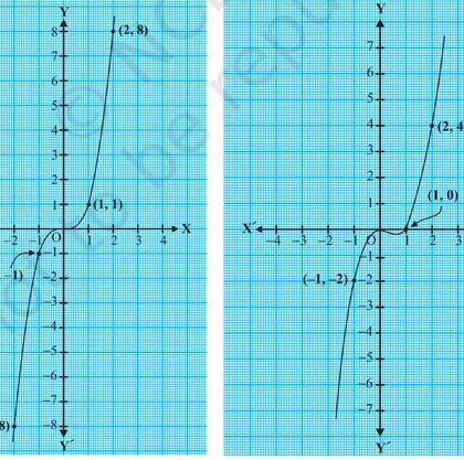
• Cubic polynomial: Degree 3, e.g. x^3 - 2x + 1. Graph has an S-like shape.
• Quartic and higher: Degree 4, 5, ... with more complex shapes.

Special case — Zero polynomial: The polynomial 0 (all coefficients zero). Its degree is undefined or sometimes taken as minus infinity; treat it separately in classification.

Important properties

• The degree of the sum or product of polynomials: deg(P + Q) ≤ max(deg P, deg Q), deg(P·Q) = deg P + deg Q (if neither is zero).
• A polynomial of degree n has at most n distinct real zeros (roots).

These classifications help in solving equations, sketching graphs, and modelling real situations where relationships between quantities follow polynomial expressions.

Definition: A zero (or root) of a polynomial p(x) is a number r such that p(r) = 0. Graphically, zeros are the x‑coordinates where the polynomial curve meets the x‑axis.

Factor Theorem: If r is a zero of p(x), then (x − r) is a factor of p(x). Conversely, if (x − r) is a factor, then r is a zero.

Remainder Theorem: When p(x) is divided by (x − c), the remainder is p(c). So p(c) = 0 exactly when (x − c) is a factor.

Multiplicity: If (x − r)^k divides p(x) but (x − r)^k+1 does not, r is a root of multiplicity k. Multiplicity affects the graph: odd multiplicity => curve crosses the x‑axis; even multiplicity => curve touches and bounces off the axis.

Fundamental Theorem of Algebra: A polynomial of degree n (with complex coefficients) has exactly n roots in the complex numbers, counted with multiplicity. For real polynomials some roots may be complex (non‑real) and appear in conjugate pairs.

How to find zeros (common methods):

• Factorization: express p(x) as product of linear/quadratic factors.
• Quadratic formula: for ax²+bx+c=0, use x = [−b ± sqrt(b² − 4ac)]/(2a).
• Synthetic division or polynomial long division to reduce degree once a root is known.
• Graphing or numerical methods for difficult cases.

Relation between coefficients and zeros (Vieta's formulas): For p(x)=a_nxⁿ + a_n−1xⁿ⁻¹ + ... + a₁x + a₀, with roots r₁, r₂, …, r_n (counted with multiplicity):

• Sum of roots = r₁ + r₂ + ... + r_n = −a_n−1/a_n.
• Product of roots = r₁·r₂·...·r_n = (−1)ⁿ a₀/a_n.

Discriminant (quadratic): D = b² − 4ac determines nature of roots: D > 0 two distinct real roots, D = 0 one repeated real root, D < 0 two complex conjugate roots.

Interpretation and checking: After finding candidate roots, substitute into p(x) to verify p(r) = 0. If a root is known, divide p(x) by (x − r) to reduce degree and find remaining roots.

What is a polynomial? A polynomial in a variable x is an expression of the form a_n xⁿ + a_{n-1} x^n-1 + ... + a_1 x + a_0 where coefficients a_i are real numbers and n is a non-negative integer. The term with the highest power n gives the degree of the polynomial. (The zero polynomial has no well-defined degree.)

Basic operations:

• Addition / Subtraction: Add or subtract corresponding coefficients of like powers (terms with same power of x). The degree of the sum is at most the maximum of the degrees of the addends; cancellation can make it smaller.
• Multiplication: Use the distributive law: multiply every term of one polynomial by every term of the other and collect like terms. The degree of the product equals the sum of the degrees of the factors (unless cancellation reduces it).
• Division: Polynomial long division (or synthetic division for divisors of form x - a) produces a quotient and a remainder. Division algorithm:
  dividend = divisor × quotient + remainder, where degree(remainder) < degree(divisor).
• Remainder theorem: If a polynomial f(x) is divided by (x − a), the remainder is f(a). Useful for quick evaluation and checking factors.
• Factor theorem: (x − a) is a factor of f(x) ⇔ f(a) = 0. This helps factor polynomials to find roots.

Techniques and shortcuts: Use algebraic identities (binomial square, difference of squares, sum/difference of cubes) to multiply or factor polynomials quickly. For dividing by linear factors, synthetic division saves work.

Worked idea (short): To add 3x² + 5x − 2 and 2x² − 4x + 7, line up like terms: (3x²+2x²) + (5x−4x) + (−2+7) = 5x² + x + 5.

Why it matters (applications): Polynomials model areas, volumes, cost/revenue functions, trajectories (quadratics), and are building blocks for algebra, calculus and many applied problems.

Statement. For any two polynomials p(x) (dividend) and g(x) (divisor) with g(x) ≠ 0, there exist unique polynomials q(x) (quotient) and r(x) (remainder) such that

p(x) = g(x)·q(x) + r(x),

where either r(x) = 0 or deg r(x) < deg g(x). This is called the Division Algorithm for Polynomials.

Why it holds (idea). By repeated subtraction of suitable multiples of g(x) from p(x) (just like integer long division) we lower the degree step by step. When the remaining polynomial has degree less than deg g(x), we stop — that remainder is r(x) and all subtractions collected form q(x). Uniqueness follows because if two different pairs (q,r) and (q',r') satisfied the relation, subtracting gives (q−q')·g(x) = r'−r; degree considerations force q=q' and r=r'.

How to perform the division (long division — procedure).

1. Arrange both p(x) and g(x) in descending powers of x, inserting zero-coefficient terms if necessary.
2. Divide the leading term of p(x) by the leading term of g(x) to get the first term of q(x).
3. Multiply g(x) by that term and subtract from p(x); the result is a new smaller-degree polynomial.
4. Repeat steps 2–3 until the remaining polynomial has degree less than deg g(x). That remainder is r(x).

Special useful results.

• Remainder Theorem: If you divide p(x) by (x − a), the remainder is p(a). So p(x) = (x − a)·q(x) + p(a).
• Factor Theorem: (x − a) is a factor of p(x) iff p(a) = 0.

Practical notes. For linear divisors x − a, synthetic division (a tabular method) is faster than polynomial long division. For higher-degree divisors use long division or compare coefficients after multiplication.

Checks and uniqueness. After division, verify by computing g(x)·q(x) + r(x) and confirming it equals p(x). The quotient and remainder are unique for the given p and g.

Statement. If a polynomial f(x) is divided by (x − a), then the remainder is f(a).

Short proof. By polynomial division, f(x) = (x − a)·q(x) + r(x), where the degree of r(x) < degree of (x − a) = 1. Hence r(x) is a constant r. Put x = a to get f(a) = r. Thus remainder = f(a).

Consequences and extensions.

• Factor Theorem: (x − a) is a factor of f(x) if and only if f(a) = 0.
• If the divisor is (ax − b) (a ≠ 0), you can rewrite it as a(x − b/a). The remainder when f(x) is divided by (ax − b) equals f(b/a).
• For a divisor g(x) of degree n, the remainder is a polynomial r(x) of degree < n. To find r(x) (of degree < n) write f(x) = g(x)·Q(x) + r(x) and determine the coefficients of r(x) by equating coefficients or by substituting n distinct values of x (for example, the n roots of g(x) if available).

How this helps: It gives a quick way to find the remainder without doing full long division, helps test if a linear factor divides a polynomial (factor theorem), and is a standard tool for factoring and root-finding of polynomials in Class 10 problems.

What is a factor of a polynomial? A polynomial q(x) is a factor of a polynomial p(x) if there exists a polynomial r(x) such that p(x) = q(x)·r(x). In particular, a linear polynomial (x − a) is a factor of p(x) if p(x) can be written as (x − a)·g(x).

Remainder Theorem (brief): If a polynomial p(x) is divided by (x − a), the remainder is p(a).

Factor Theorem (statement): For a polynomial p(x), (x − a) is a factor of p(x) if and only if p(a) = 0. Equivalently, a is a zero/root of p(x) exactly when (x − a) divides p(x).

Why it works (short proof idea): By division algorithm, p(x) = (x − a)·q(x) + r, where r is a constant. Putting x = a gives p(a) = r. So p(a) = 0 ⇔ r = 0 ⇔ p(x) is exactly divisible by (x − a).

Use of Factor Theorem in factorization: To factor a polynomial with integer coefficients, we

1. Guess a possible rational root a (by Rational Root Test: possible roots are factors of constant term divided by factors of leading coefficient).
2. Evaluate p(a). If p(a) = 0, then (x − a) is a factor.
3. Divide p(x) by (x − a) (long division or synthetic division) to get a lower-degree polynomial q(x).
4. Factor q(x) further (repeat the process) until p(x) is expressed as product of irreducible factors (linear or irreducible quadratics).

Types of factorization often used in Class 10: factoring quadratics (ax^2 + bx + c) into linear factors using zeroes or the quadratic formula; factoring cubic polynomials using the factor theorem and synthetic division; factorization by grouping for polynomials with four terms.

Multiplicity of roots: If p(a) = p'(a) = ... = p^{(k-1)}(a) = 0 but p^{(k)}(a) ≠ 0, then (x − a)^k is a factor and a is a root of multiplicity k. Graphically, multiplicity affects whether the curve crosses (odd multiplicity) or touches and turns (even multiplicity) at x = a.

Practical tips: Start trying small integer divisors of the constant term (±1, ±2, …). Use synthetic division for quick division. Check for common factors first. For quadratics, use sum-product relations (sum of roots = −b/a, product = c/a) to help factor.

Definition: For a polynomial p(x) = a_n x^n + a_{n-1} x^{n-1} + ... + a_1 x + a_0 (a_n ≠ 0), a zero (or root) is a number r such that p(r)=0. If the zeros are r1, r2, ..., rn (counted with multiplicity), the polynomial can be written as a_n(x - r1)(x - r2)...(x - rn).

Vieta's relations (core idea): Expanding a_n(x - r1)(x - r2)...(x - rn) and comparing coefficients with a_n x^n + a_{n-1} x^{n-1} + ... + a_0 gives symmetric relations between the zeros and the coefficients. In particular:

• Sum of the zeros: r1 + r2 + ... + rn = -a_{n-1}/a_n.
• Sum of products of zeros taken two at a time: Σ_{i
• More generally, the k-th elementary symmetric sum of the zeros equals (-1)^k a_{n-k}/a_n.
• Product of all zeros: r1 r2 ... rn = (-1)^n a_0 / a_n.

Quadratic special case: For ax^2 + bx + c (a ≠ 0) with zeros α and β,

• α + β = -b/a
• αβ = c/a

These give quick checks and help reconstruct a quadratic if zeros are known: a(x - α)(x - β) = ax^2 - a(α + β)x + aαβ.

Consequences and useful facts:

• If coefficients are real, non-real complex zeros occur in conjugate pairs.
• For a quadratic ax^2 + bx + c, the axis of symmetry x-coordinate is (α + β)/2 = -b/(2a); the vertex y-value can be expressed using coefficients or discriminant.
• The sign of the product of real zeros equals the sign of c/a for a quadratic; zero constant term a_0 = 0 implies x = 0 is a root.
• Vieta's relations let you find one root when others are known, or check correctness of factorization.

Why it works (brief derivation): Write p(x)=a_nΠ(x - r_i). Expanding, the coefficient of x^{n-1} is -a_n Σ r_i, so a_{n-1} = -a_n Σ r_i. Similarly, the constant term is a_n (-1)^n Π r_i, so a_0 = a_n (-1)^n Π r_i. This yields the formula pattern above.

Idea: If α, β, γ, ... are the zeros (roots) of a polynomial, then the polynomial (up to a nonzero constant factor k) can be written as the product of linear factors (x−α)(x−β)(x−γ).... The degree of the polynomial equals the number of zeros counting multiplicity.

Steps to form a polynomial from given zeros:

• Write the factor for each zero: (x − zero). If a zero has multiplicity m, include that factor m times.
• Multiply the factors to get the polynomial. Optionally choose a constant k (often 1) so the polynomial has the desired leading coefficient or integer coefficients.
• If zeros are fractions, clear denominators by multiplying by an appropriate k to get integer coefficients.
• If a complex number a + bi (b ≠ 0) is given as a zero and you want a polynomial with real coefficients, include its conjugate a − bi as a zero too (complex roots occur in conjugate pairs).

Relations (Vieta's formulas) for coefficients: For a monic polynomial with zeros α, β (quadratic): x^2 − (α+β)x + αβ. For cubic with zeros α, β, γ: x^3 − (α+β+γ)x^2 + (αβ+βγ+γα)x − αβγ.

Common pitfalls: Remember multiplicity (even multiplicity => the graph touches the x-axis; odd multiplicity => it crosses). When zeros are rational fractions, multiply by the LCM of denominators to avoid fractional coefficients.

Overview
In Class 10 Polynomials, 'Applications and Problem Solving' means modeling real situations by polynomials, using algebraic tools (factorisation, division algorithm, remainder and factor theorems) to solve the model and interpreting results in context. Typical problems ask for unknown lengths, times, counts, costs, or to check whether a given expression is a factor or to find remainders quickly.

Common steps to solve application problems

• Understand the situation and choose a variable (say x) for the unknown quantity.
• Translate relationships into an algebraic expression or polynomial.
• Simplify to get a polynomial equation (often quadratic or cubic).
• Use factorisation, the remainder theorem, the factor theorem, or division algorithm to solve or reduce the polynomial.
• Check roots for extraneous or non-physical values (negative lengths, etc.) and interpret the solution in context.

Key techniques and how they help

• Factorisation: converts a polynomial equation into simpler linear factors so you can find roots quickly.
• Remainder theorem: evaluate P(a) to get remainder when P(x) is divided by (x − a) — faster than long division.
• Factor theorem: if P(a)=0 then (x − a) is a factor; used to test and factor polynomials and find unknown coefficients.
• Division algorithm: P(x)=D(x)Q(x)+R(x) is used when dividing polynomials; R(x) has smaller degree than D(x).

Real-life contexts: area/perimeter problems (lengths expressed as linear expressions lead to quadratic area), profit/cost/revenue modeled by polynomials, mixture problems, sequence sums, and design/layout partitioning (dividing land, tiling), and checking feasibility constraints (non-negative roots).

Tips

• Always write units and check whether roots make sense physically.
• If you obtain a polynomial with degree > 2, try rational root test or factor by grouping.
• Sketching the graph of the polynomial helps visualize number and multiplicity of real roots.