Overview
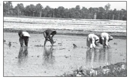
This chapter examines land as a limited and vital resource in India and the role of agriculture in the economy. It introduces types of land use (net sown area, forest, pasture, land under non-agricultural uses, cultivable wasteland), patterns and regional variations in land use, and problems of land degradation, fragmentation and declining soil health. The chapter explains the structure and types of farming in India (subsistence, commercial, plantation, mixed), cropping seasons (kharif, rabi, zaid), cropping patterns, and allied activities (animal husbandry, fisheries, forestry). It covers major inputs and technologies — irrigation, fertilisers, high-yielding varieties, mechanisation — and evaluates the Green Revolution, its benefits and ecological costs. Institutional issues such as land tenure, land reforms (abolition of intermediaries, land ceiling, consolidation, tenancy reforms), and newer approaches (cooperatives, contract farming, watershed management, organic farming) are discussed. The chapter highlights environmental problems (salinisation, waterlogging, soil erosion, deforestation) and sustainable land management practices (soil conservation, agroforestry, crop…
Learning Objectives
- Define land resources and classify types of land use (forests, permanent pastures, cultivable land, fallow land, net sown area).
- Explain the concept of land use pattern and cropping intensity, and calculate cropping intensity from given data.
- Describe major types of agriculture (subsistence, commercial, intensive, extensive, plantation, mixed, shifting) and their spatial distribution in India.
- Compare and contrast intensive subsistence farming and commercial grain farming with regional examples.
- Explain the Green Revolution: its technological components (high-yielding varieties, irrigation, fertilizers) and outcomes.
- Assess the socio-economic and environmental impacts of the Green Revolution and modern agricultural practices.
- Analyse physical, economic and socio-political factors that influence land use change and agricultural productivity.
- Identify causes and consequences of land degradation, soil erosion and desertification, and prioritise their impacts on livelihoods.
Topics in this chapter
27 topics · tap a topic title to jump straight to it.
Introduction to Land Resources
What are land resources?
Land is a finite natural resource that supports all terrestrial life and human activities. It includes the Earth's surface used for agriculture, forestry, settlements, industry, transport, recreation and wilderness. In geography, 'land resources' refer to the area of the Earth's surface available for productive uses, its physical attributes (soil, slope, drainage), and the ways humans use and manage it.
Major components of land resources
- Net sown area (NSA): Area sown with crops at least once in a year.
- Gross cropped area (GCA): Total area sown counting areas sown more than once (GCA ≥ NSA).
- Forest land: Areas under natural and planted forests.
- Permanent pastures and grazing land: Used for livestock.
- Fallow land: Current fallow (left for one year) and other fallows (left for more than one year but less than five).
- Land not available for cultivation: Settlements, roads, rocky waste, deserts, water bodies, glaciated areas.
Determinants of land use and quality
- Physical factors: soil type, slope, drainage, climate, vegetation and water availability.
- Technological factors: irrigation, fertilizers, mechanisation, crop varieties.
- Socio-economic factors: population pressure, land tenure, market access, urbanisation and policies.
Problems affecting land resources
- Land degradation: Soil erosion (water/wind), salinisation, alkalisation and nutrient depletion reduce productive capacity.
- Desertification: Expansion of arid conditions (e.g., overgrazed or deforested drylands).
- Urbanisation and loss of agricultural land: Conversion of fertile land into built-up areas.
- Fragmentation: Subdivision of holdings reduces viability of farming operations.
Conservation and sustainable management
- Soil conservation: contour ploughing, terracing, strip cropping, check dams and mulching.
- Watershed management: capture and recharge of water, afforestation and community management.
- Crop management: crop rotation, intercropping, agroforestry and integrated nutrient management.
- Land-use planning: zoning, protection of prime agricultural land, urban growth boundaries and rehabilitation of degraded lands.
Why this matters (link to agriculture and food security)
Land resources determine the area available for cultivation, intensity of cropping and long‑term sustainability of food production. Efficient, equitable and ecological use of land is central to rural livelihoods, biodiversity and climate resilience.
Key terms to remember: Net sown area (NSA), Gross cropped area (GCA), Cropping intensity, Fallow land, Land degradation, Watershed management.
- Punjab and Haryana — high cropping intensity and multiple cropping due to irrigation (Green Revolution).
- Shifting cultivation (jhum) in northeast India — traditional slash-and-burn leading to periodic fallow and local deforestation.
- Desertification in parts of Rajasthan (Thar) due to overgrazing, deforestation and poor irrigation management.
- Coastal land erosion in Sundarbans — loss of agricultural and mangrove land from sea-level rise and storm surges.
- Land reclamation in parts of Gujarat (wetland and coastal reclamation) and urban expansion converting peri‑urban farmland (e.g., around Delhi and Mumbai).
- Land use percentage for a category = (Area of that category / Total Geographical Area) × 100
- Cropping intensity (%) = (Gross Cropped Area (GCA) / Net Sown Area (NSA)) × 100
- Per capita availability of land = Total Geographical Area / Total Population
- Annual rate of change in area (%) = [(Area_year2 − Area_year1) / Area_year1] × (100 / Number_of_years_between)
- Gross Cropped Area (GCA) = Sum of areas sown for all crops in the year (includes multiple cropping); NSA ≤ GCA
Land Use Classification
What is Land Use Classification?
Land use classification is the systematic categorization of a region’s land according to its current primary use — for example agriculture, forest, settlements, grazing, or wasteland. It helps planners, geographers and policymakers understand how land is utilised, monitor changes, and plan sustainable development.
Land use vs Land cover
Land cover describes the physical surface (forest, water, built-up), while land use describes the human purpose for which the land is used (cropping, grazing, conservation, residential). A single land cover type (e.g., grassland) can have different land uses (pasture, recreation).
Main categories used in Indian land-use statistics
The commonly used categories (as in national land-use statistics) are:
- Forest: Areas under natural or planted forests, wildlife reserves and mangroves.
- Land put to non-agricultural uses: Urban areas, roads, industrial sites, reservoirs and other built-up uses.
- Barren and unculturable land: Areas unsuitable for cultivation (rocky, desert, high mountains).
- Permanent pastures and grazing land: Natural grasslands and meadows used for grazing livestock.
- Land under miscellaneous tree crops and groves: Orchards, coffee, rubber, tea — tree crops not included in net sown area.
- Culturable waste land: Degraded or temporarily unusable lands that can be cultivated after improvement.
- Fallow lands: Agricultural lands left uncropped for one or more seasons (current fallow, other fallow).
- Net sown area (NSA): Land sown at least once in the year, representing actively cropped area.
Why classify land?
Classification supports: resource accounting, agricultural planning (crop zones, irrigation), urban planning, forestry management, environmental protection, and monitoring land conversion (e.g., farm to city).
How land use is measured
Methods include field surveys (land records), cadastral maps, and increasingly remote-sensing and GIS which allow temporal monitoring (decadal change in forest cover, urban sprawl, reclamation of fallow lands).
Key processes and trends
- Urbanisation: conversion of agricultural land to built-up uses (e.g., peri-urban expansion around Delhi, Mumbai).
- Deforestation and afforestation: forest area declines or increases regionally (e.g., clearing for agriculture vs plantation drives).
- Desertification and land degradation: increases barren/culturable waste in arid regions (e.g., parts of Rajasthan).
- Agricultural intensification: increase in gross cropped area via multiple cropping, higher cropping intensity in irrigated states (Punjab, Haryana).
Implications for policy and sustainability
Balanced land use classification helps identify areas for conservation, agricultural investment, urban containment policies, soil and water conservation, and disaster risk reduction.
- Punjab and Haryana: High net sown area and high cropping intensity due to irrigated agriculture (wheat–rice cropping).
- Rajasthan (western parts): Large share of barren and unculturable land (Thar Desert), limited cultivable area.
- Arunachal Pradesh and Northeast: High forest cover and shifting cultivation pockets; forest land dominates land-use statistics.
- National Capital Region (NCR): Rapid conversion of agricultural land to land put to non-agricultural uses (residential, commercial).
- Sundarbans (West Bengal): Mangrove forest classified as forest land and protected; not part of net sown area.
- Himachal Pradesh: Significant area under miscellaneous tree crops (apple orchards) and forests; limited net sown area in hilly terrain.
- Net Sown Area (NSA) = Total area sown with crops at least once in the year (hectares)
- Gross Cropped Area (GCA) = Sum of areas sown under each crop during the year (counting multiple cropping) (hectares)
- Cropping Intensity (%) = (GCA / NSA) × 100
- Land Use Percentage (%) for a category = (Area of category / Total reporting area) × 100
- Percentage of Net Sown Area in reporting area (%) = (NSA / Total reporting area) × 100
Land Use Terminology and Statistics
Land use terminology and statistics describe how land is classified and measured for planning and agricultural assessment. In India (and in CBSE Geography) land is grouped into standard categories so that area, productivity and changes over time can be compared across regions.
- Geographical area: Total area within political boundaries (state or country).
- Net sown area (NSA): Area sown at least once in a year. It shows the actual extent of agricultural activity.
- Gross cropped area (GCA): Sum of areas sown, counting each sowing separately. If a hectare is sown twice, it is counted twice in GCA. GCA reflects total cropping (including multiple cropping).
- Area sown more than once: GCA − NSA. Indicates intensity of multiple cropping.
- Cropping intensity: Degree of multiple cropping; it shows how intensively NSA is used.
- Current fallow: Land left uncropped for less than one year (temporary fallows).
- Other fallow: Land left uncropped for 1–5 years.
- Culturable waste / cultivable wasteland: Land that is cultivable but not currently cultivated (may be degraded or awaiting reclamation).
- Permanent pastures and grazing land: Used mainly for livestock grazing.
- Land put to non-agricultural uses: Settlements, industry, roads, mines, reservoirs, etc.
- Forest cover: Area under natural or planted forests (important for ecology and watershed management).
- Barren and uncultivable land: Rocky, desert or very steep lands not suitable for cultivation.
Why these statistics matter:
- Planning: Determine food security, irrigation needs and rural development priorities.
- Land management: Identify areas for reclamation (culturable waste), afforestation or protection.
- Environmental monitoring: Track loss of agricultural land to urbanization or growth of forest cover.
Important relationships: Net sown area and gross cropped area together reveal the cropping intensity and capacity to produce food. Distribution of land use categories varies widely by state: some states (like Punjab and Haryana) have high NSA and high cropping intensity, while others (like Rajasthan) have large areas of cultivable waste and barren land. Urbanization increases 'land put to non-agricultural uses', reducing agricultural land in many regions.
- Punjab and Haryana: High net sown area and very high cropping intensity due to intensive irrigation and double/triple cropping; GCA is much larger than NSA.
- Rajasthan: Large proportion of barren and uncultivable land and cultivable wasteland; lower NSA and low cropping intensity in arid regions.
- Kerala: Fragmented holdings and high use of land for tree crops and plantations; substantial area under permanent crops and multiple cropping in small holdings.
- Maharashtra (urban districts like Mumbai/Pune): Growing 'land put to non-agricultural uses' because of urban expansion and industry.
- Madhya Pradesh / Chhattisgarh: Large forest area in some districts, affecting the proportion of land available for agriculture.
- Area sown more than once = Gross Cropped Area (GCA) − Net Sown Area (NSA)
- Cropping intensity (%) = (GCA / NSA) × 100
- Percentage of any land-use category = (Area of category / Geographical area) × 100
- Net sown area proportion (%) = (NSA / Geographical area) × 100
Patterns of Land Use in India
Introduction
Patterns of land use in India describe how different parts of the country allocate land to agriculture, forests, pastures, wasteland, settlements, and other uses. These patterns reflect variations in physiography, climate, soils, irrigation, population pressure, economic development and historical policies (for example the Green Revolution).
Main land‑use categories
The usual categories used in Indian land‑use statistics are: Net Sown Area (NSA), Gross Cropped Area (GCA), Current and Other Fallow, Cultivable Waste, Land Not Available for Cultivation (built‑up, rocky, barren), Permanent Pastures and Grazing, Forests, and Miscellaneous Tree Crops/Plantations. GCA counts multiple crops on the same land; NSA counts each hectare only once.
Spatial patterns and causes
1) Irrigated vs rainfed: Northern plains (Punjab, Haryana, parts of Uttar Pradesh) and some canal command areas have high irrigation coverage and intensive multiple cropping. Eastern and north‑eastern regions are more rainfed and typically have single cropping in many districts. Southern peninsular regions show mixed patterns — intensively cultivated irrigated tracts (e.g., Krishna and Cauvery deltas) alongside dryland areas.
2) Cropping intensity (extent of multiple cropping): Highest in irrigated, fertile plains (Indo‑Gangetic plain). Low in arid and semi‑arid zones (Rajasthan, parts of Gujarat, central plateau) and in steep, forested or hilly regions.
3) Forest and tree cover: Concentrated in the Himalayan foothills, North‑East, Western Ghats, central plateau (parts of Chhattisgarh, Madhya Pradesh), and Andaman & Nicobar. Forest cover reduces the proportion of land available for cultivation but provides ecosystem services.
4) Wasteland and cultivable waste: More common in arid (Rajasthan), semi‑arid (parts of Maharashtra, Karnataka), and degraded landscapes affected by erosion and salinity. Mining areas (Jharkhand, Chhattisgarh) and deforested tracts also show high non‑cultivable land.
5) Urbanization and industrial land use: Rapid growth of cities (Delhi NCR, Mumbai, Bengaluru, Chennai, Pune) converts agricultural land to built‑up use, peri‑urban horticulture, and infrastructure.
6) Special land‑use systems: Shifting cultivation (jhum) in some north‑eastern states, plantations (tea, coffee, rubber, spices) in Kerala, Assam, Karnataka and Tamil Nadu, coastal aquaculture/prawn farms in Andhra Pradesh, West Bengal and Odisha, and dryland horticulture in parts of Maharashtra.
Temporal change drivers
Trends include a long‑term decline in proportion of land under agriculture in some regions due to urbanization and industrialization, improvement in irrigation and multiple cropping in others (increasing GCA and cropping intensity), and afforestation/reforestation programs altering forest area. Land degradation, salinization and desertification change the quality and effective availability of agricultural land.
Implications for policy and management
Understanding spatial patterns is essential for targeting irrigation investments, soil conservation, watershed management, afforestation, urban planning, and agricultural extension. Policies must be location‑specific: promoting multiple cropping and high‑value horticulture where irrigation exists; drought‑resilient crops and water harvesting in drylands; and sustainable forest management and alternatives to shifting cultivation in hilly regions.
- Punjab and Haryana: High percentage of net sown area with extensive canal and tube‑well irrigation, resulting in high cropping intensity and multiple cropping (wheat–rice systems). Example of Green Revolution impact.
- Rajasthan: Large areas of land not available for cultivation (Thar Desert) and significant cultivable wasteland; cropping limited by low rainfall and irrigation.
- North‑East (e.g., Nagaland, Meghalaya): Presence of shifting cultivation (jhum) and high forest cover; small fragmented fields and lower mechanization and irrigation.
- West Bengal (deltaic tracts) and Tamil Nadu (Cauvery delta): Intensive paddy cultivation with high cropping intensity in irrigated deltaic zones; also presence of aquaculture in coastal districts (e.g., Sunderbans fringe, coastal Andhra and Odisha).
- Maharashtra (Deccan plateau): Large areas of dryland farming, high incidence of cultivable waste and fallows in drought‑prone districts; rise of cash crops (cotton, soybean) and horticulture in better‑irrigated tracts.
- Urban corridors (Delhi NCR, Mumbai–Pune–Bengaluru): Rapid conversion of agricultural land to built‑up land, peri‑urban horticulture and industrial uses.
- Net Sown Area (NSA) = Total area sown with crops (each hectare counted once)
- Gross Cropped Area (GCA) = Sum of area sown under all crops (areas sown more than once counted each time)
- Cropping Intensity (%) = (GCA / NSA) × 100
- Percentage share of a land‑use category = (Area of category / Total geographical area) × 100
- Irrigation intensity (%) = (Irrigated area / NSA) × 100 (or proportion of NSA that is irrigated)
Soil Types of India
Overview: Soils of India are diverse due to variations in parent rock, relief, climate, vegetation and time. Major soil types discussed in Class 12 Geography (Land Resources and Agriculture) are: Alluvial, Black (Regur), Red, Laterite, Desert, Saline & Alkaline (Usar/Kallar/Reh), Peaty & Marshy and Mountain/Forest soils. Each has characteristic profile, fertility and crop suitability.
Alluvial Soils
Distribution: Indo-Gangetic-Brahmaputra plains and river deltas, parts of coastal plains. Composition: mixed clay, silt and sand; very fertile and deep. Types: Khaddar (new, fine silts, floodplain) and Bhangar (older alluvium with kankar/calcareous nodules). Good for rice, wheat, sugarcane, pulses.
Black (Regur) Soils
Distribution: Deccan plateau — Maharashtra, Madhya Pradesh, Gujarat, parts of Andhra Pradesh and Karnataka. Character: rich in clay, high moisture retention, dark due to organic matter and iron compounds; ideal for cotton (called 'black cotton soil'), also suited to groundnut, wheat, millets.
Red Soils
Distribution: Peninsular plateau — Tamil Nadu, Karnataka, eastern Maharashtra, Odisha, Chhattisgarh. Character: Reddish due to iron oxides, low humus, porous, often acidic and low in nitrogen/phosphorus. Grown crops: millets, pulses, oilseeds, cotton (with manuring/irrigation).
Laterite Soils
Distribution: High rainfall and high temperature regions — Western Ghats, eastern ghats, parts of Assam, Kerala. Character: intense leaching, rich in iron and aluminium oxides, poor in bases and organic matter, often hard when dry. Used for plantation crops (tea, coffee, cashew) after enrichment.
Desert Soils
Distribution: Rajasthan (Thar), parts of Gujarat and Haryana. Character: sandy, low organic matter, poor water retention, frequent salinity and wind erosion. Vegetation is sparse; crops need irrigation (millets, barley, drought-tolerant oilseeds).
Saline and Alkaline Soils (Usar, Kallar, Reh)
Distribution: arid and semi-arid tracts, poorly drained areas, some coastal areas. Character: white efflorescence of salts, pH high (alkaline), reduces crop growth. Reclamation by proper drainage, gypsum application and leaching.
Peaty and Marshy Soils
Distribution: waterlogged areas, deltas (parts of Sunderbans), coastal Kerala backwaters. Character: high organic matter, waterlogged, acidic; after draining and manuring can be productive for paddy and plantation crops.
Mountain / Forest Soils
Distribution: Himalayan and other hill areas. Character: shallow, coarse, acidic in high rainfall regions, rich humus in colder climates. Terraced agriculture practiced; crops include fruits, vegetables, plantation crops, coarse cereals.
Factors influencing soil formation: parent rock, climate (temperature & rainfall), relief/topography, biological activity (vegetation & microbes), time and human activity (irrigation, deforestation).
Problems and management: soil erosion (by water & wind), salinisation, nutrient depletion, waterlogging. Management includes contour bunding, afforestation, crop rotation, balanced fertilization, organic manuring, drainage & gypsum for alkali soils, and conservation agriculture.
- Alluvial soil: Wheat and sugarcane cultivation in Punjab, Haryana and western Uttar Pradesh (Indo-Gangetic plain).
- Black (Regur) soil: Cotton cultivation in Vidarbha and Marathwada (Maharashtra); also suitable for soybean in Madhya Pradesh.
- Red soil: Millets and pulses in Karnataka and Tamil Nadu (rainfed agriculture).
- Laterite soil: Tea and coffee plantations along the Western Ghats (Kerala, Karnataka).
- Desert soil: Pearl millet (bajra) and drought-resistant oilseeds grown in parts of Rajasthan with irrigation; sand dune stabilization with afforestation.
- Saline/alkaline soil: Reclamation projects in parts of Uttar Pradesh and Haryana use gypsum and sub-surface drainage to reduce soil salinity.
- Soil moisture (%) = (Mass of wet soil – Mass of dry soil) / Mass of dry soil × 100
- Bulk density (g/cm³) = Mass of dry soil (g) / Volume of soil (cm³)
- Porosity (%) = [1 – (Bulk density / Particle density)] × 100 (Particle density ≈ 2.65 g/cm³ for mineral soils)
- Available water capacity (approx) = Field capacity – Permanent wilting point (both expressed as % by volume)
- Soil organic carbon (%) from loss-on-ignition or lab methods; Organic matter (%) ≈ Organic carbon (%) × 1.724 (Van Bemmelen factor)
Soil Formation and Properties
Soil Formation and Properties
Definition: Soil is a natural body composed of mineral particles, organic matter, water, air and living organisms — formed at the interface of lithosphere, atmosphere, hydrosphere and biosphere. It supports plant life and human activities.
How soil forms (Factors and Processes)
Soil formation is governed by five principal factors (mnemonic: CLORPT):
- Climate — temperature and rainfall control physical and chemical weathering and organic decomposition. (Example: monsoon climates produce deep, leached soils.)
- Organisms — plants, microbes and animals add organic matter, mix the soil and accelerate mineral breakdown.
- Relief (topography) — slope and aspect affect erosion, drainage and soil depth.
- Parent material — the rock or sediment from which soil develops (e.g., granite, basalt, alluvium) determines mineralogy and texture.
- Time — pedogenesis is slow; older soils are more developed and show distinct horizons.
Key processes: weathering (physical, chemical, biological), eluviation (leaching from upper horizons), illuviation (accumulation in lower horizons), humification (formation of humus), podzolization, laterization, salinization and calcification.
Soil Profile and Horizons
Typical horizons: O (organic), A (topsoil, mineral + humus), E (eluviation layer, sometimes present), B (subsoil — accumulation of clay, oxides), C (partly weathered parent rock), R (bedrock). The profile reflects history and processes.
Properties of Soil
Physical properties:
- Texture: relative proportions of sand, silt and clay. Texture controls water retention, aeration and root penetration. (See soil texture triangle.)
- Structure: the arrangement of soil particles into aggregates (crumb, blocky, platy) — influences porosity and root growth.
- Bulk density and Porosity: indicate compaction and pore space for air/water.
- Water retention and available water: field capacity vs permanent wilting point determine how much water plants can use.
- Colour: indicates organic matter (darker soils), drainage/oxidation (red/yellow from iron oxides), or gleying in waterlogged soils.
Chemical properties:
- pH: acidity/alkalinity affects nutrient availability (most crops: pH 5.5–7.5).
- Organic matter / Organic carbon: improves structure, nutrient and water retention.
- Cation Exchange Capacity (CEC): ability to hold and exchange nutrient cations (Ca2+, Mg2+, K+, NH4+).
- Base saturation: proportion of exchange sites occupied by basic cations — indicates fertility.
- Salinity and sodicity: presence of soluble salts or excess sodium that reduce crop productivity.
Biological properties: soil biota (bacteria, fungi, earthworms) drive decomposition, nutrient cycling and aggregate formation; root activity and rhizosphere processes are crucial.
Soil Types (brief, with Indian examples)
- Alluvial soils: fertile, varied texture — Indo-Gangetic plain (rice, wheat).
- Black (Regur) soils: high clay, high moisture retention — Deccan plateau, ideal for cotton.
- Red soils: iron-rich, well-drained, lower in organic matter — parts of Tamil Nadu, Andhra Pradesh.
- Laterite soils: leached, rich in iron and aluminium — Western Ghats, used for plantation crops.
- Arid soils: saline, sandy/gravely — Rajasthan, require irrigation and reclamation.
- Mountain/Forest soils: shallow, rich in humus in temperate/forest zones — Himalayan regions.
Practical importance and management
Understanding soil properties guides crop selection, irrigation, fertiliser use and conservation: e.g., adding organic matter improves structure and water holding; gypsum ameliorates sodic soils; contour bunding reduces erosion on slopes.
Summary: Soil is the product of climate, organisms, relief, parent material and time acting through weathering and biological processes. Its physical, chemical and biological properties determine land use, productivity and management strategies.
- Indo-Gangetic plain: deep alluvial soils supporting intensive wheat–rice cropping due to high fertility and good water retention.
- Deccan Plateau: black (regur) soils derived from basalt with high clay content, good moisture retention — ideal for cotton.
- Western Ghats and Ghats foothills: laterite soils formed under high rainfall and temperature, used for plantation crops like tea and cashew after management.
- Rajasthan: arid soils with high salinity and low organic matter — require irrigation, drainage and soil reclamation (leaching salts, gypsum application).
- Himalayan slopes: shallow mountain soils rich in humus in forested zones but thin and prone to erosion — need terrace farming and afforestation.
- Bulk density (ρb) = mass of oven-dry soil / total soil volume (g/cm3 or Mg/m3).
- Porosity (%) = (1 - ρb / ρs) × 100, where ρs is particle density (~2.65 g/cm3 for mineral soils).
- Available water (AW) = Field capacity (FC) - Permanent wilting point (PWP) (usually in % or mm of water per depth).
- Organic matter (OM) ≈ Organic carbon (OC) × 1.724 (Van Bemmelen factor). Thus OC = OM / 1.724.
- Base saturation (%) = (Sum of exchangeable basic cations (Ca2+ + Mg2+ + K+ + Na+) / CEC) × 100.
Land Degradation and Soil Erosion
Introduction
Land degradation is the decline in land quality caused by human activities and natural processes that reduce its productivity and ecosystem services. Soil erosion is a major form of land degradation: the detachment and removal of the topsoil by water, wind, ice or human activity. Together they threaten food security, water quality, biodiversity and livelihoods.
Causes
- Natural factors: heavy rainfall, steep slopes, floods, and wind in arid zones.
- Human factors: deforestation, overgrazing, improper agricultural practices (monoculture, lack of crop cover, ploughing along slope), urbanisation, mining, and poor irrigation (salinisation, waterlogging).
Processes and Types of Soil Erosion
- Sheet erosion: removal of a thin uniform layer of soil by raindrop impact and runoff.
- Rill erosion: runoff concentrates to form small channels (rills) that are removable by normal cultivation.
- Gully erosion: larger concentrated flows cut deep channels that cannot be removed by ordinary tillage.
- Wind erosion: detachment and transport of fine soil particles by wind (common in dry, sandy soils).
- Landslides and mass wasting: slope failure often accelerated by removal of vegetation and increased water infiltration.
Impacts
- Loss of fertile topsoil and soil organic matter → reduced crop yields and increased fertiliser needs.
- Reduced water infiltration and groundwater recharge; increased surface runoff and flooding.
- Soil salinity and waterlogging from poor irrigation → converting arable land to unproductive land.
- Siltation of reservoirs, canals and riverbeds → reduced storage and navigation problems.
- Biodiversity loss and desertification in extreme cases.
Prevention and Management (Soil Conservation)
- Vegetative measures: afforestation, agroforestry, cover crops, mulching, contour hedgerows.
- Agronomic practices: contour ploughing, terracing, strip cropping, minimum/no-till, crop rotation.
- Engineering structures: check dams, gully plugs, retention basins, bunds and terraces.
- Irrigation management: proper drainage, leaching salts, avoid waterlogging; use of efficient irrigation methods.
- Policy and community measures: land-use planning, controlled grazing, farmer education and compensation schemes.
Assessment and Indicators
Soil loss is commonly expressed in tonnes per hectare per year (t ha–1 yr–1). Land degradation assessment combines soil loss rates, salinity/waterlogging maps, vegetation cover change (NDVI), and socio-economic indicators (cropping intensity, population pressure).
Short note on Reversibility
Some forms of degradation (topsoil loss, salinisation) are difficult and costly to reverse and may take decades to restore; prevention is therefore more cost-effective than remediation.
- Dust Bowl (USA, 1930s): severe wind erosion and loss of topsoil caused by drought and removal of native grasses combined with intensive ploughing—classic example of how poor land management can create ecological and socio-economic disaster.
- Himalayan deforestation and landslides: removal of forest cover for agriculture, road-building and urban expansion has increased slope instability and soil erosion, leading to frequent landslides and sedimentation of rivers.
- Indo-Gangetic Plain (India): intensive monoculture, excessive tillage and groundwater exploitation have led to declining soil organic matter, compaction and localised erosion despite generally low slope—requires improved conservation practices.
- Thar Desert expansion and desertification (Rajasthan, India): overgrazing, fuelwood removal and unsustainable land use have contributed to loss of soil cover and outward spread of degraded land.
- Sunderbans and coastal erosion: sea-level rise, cyclones and reduced sediment supply from upstream have increased coastal erosion, mangrove loss and salt intrusion affecting agriculture and fisheries.
- Universal Soil Loss Equation (USLE): A = R × K × LS × C × P, where - A = average annual soil loss (t ha⁻¹ yr⁻¹) - R = rainfall erosivity factor (MJ mm ha⁻¹ h⁻¹ yr⁻¹ or similar) - K = soil erodibility factor (t ha h ha⁻¹ MJ⁻¹ mm⁻¹) - LS = topographic factor (slope length × slope steepness) - C = cover-management factor (dimensionless, 0–1) - P = support practice factor (dimensionless, 0–1)
- Percent land degraded: % Degraded = (Area of degraded land / Total area) × 100
- Gully volume (estimate): V = A × d, where - V = volume of soil removed (m³) - A = plan area of gully (m²) - d = average depth (m) (Convert volume to mass using soil bulk density, e.g., mass = V × bulk density (t m⁻³))
- Soil loss rate unit conversion: if A (t ha⁻¹ yr⁻¹) is known, total annual soil loss = A × area (ha).
Soil Conservation Measures
Definition & Importance: Soil conservation comprises practices that prevent soil erosion, restore degraded soils and maintain soil fertility so that land remains productive. Conserving soil sustains crop yields, prevents siltation of reservoirs, reduces flood risk and preserves ecological health.
Causes of Soil Degradation: Major causes include water erosion (runoff on slopes), wind erosion (dry, exposed soils), deforestation and overgrazing, intensive tillage, loss of organic matter, salinisation and alkalinity (poor irrigation/drainage) and contamination.
Types of Measures
- Agronomic measures (land-management practices): contour ploughing and contour bunding, strip cropping and crop rotation, cover crops and green manures, mulching, reduced or zero tillage (conservation tillage), intercropping and agroforestry. These reduce runoff, increase infiltration and improve organic matter.
- Engineering measures (structural works): terracing on steep slopes, graded bunds and field bunding, check dams and gully plugs, stone lines and contour trenches, percolation pits and rainwater harvesting structures—all to slow runoff, trap sediment and increase groundwater recharge.
- Biological measures (vegetation-based): afforestation, shelterbelts (windbreaks), grass sodding of gullies (e.g., vetiver hedgerows), riparian buffer strips alongside streams to filter sediments and prevent bank erosion.
- Soil chemical & reclamation measures: reclamation of saline/alkaline soils by gypsum application and leaching, subsurface drainage, liming acidic soils, integrated nutrient management and regular soil testing to guide fertilizer use.
- Policy & community approaches: watershed development programs, community-based land management, afforestation campaigns, and employment-linked schemes (e.g., MGNREGA tasks in India) that build structures and restore degraded catchments.
How they work (summary): Structural measures reduce the velocity of runoff so sediment is deposited; vegetative measures bind soil, reduce raindrop impact and increase infiltration; agronomic measures keep the soil covered and improve organic matter and structure; reclamation corrects chemical imbalances so plants can re-establish.
Brief note on estimating erosion: The Universal Soil Loss Equation (USLE) is a commonly used empirical model to estimate average annual soil loss and to plan conservation: A = R × K × LS × C × P (A = estimated soil loss per unit area). Each factor guides which measures will be most effective (for example, reduce C by cover crops; reduce LS by terracing; alter P by contouring/bunding).
Outcomes: Properly chosen and combined measures reduce soil loss, increase productivity and resilience to drought/flood, conserve water, and reduce downstream siltation and damage.
- Ralegan Siddhi (Maharashtra): community-led watershed and soil-conservation works (contour trenches, check dams, tree planting) that restored groundwater and agricultural productivity.
- Terracing in the Himalayan and North-Eastern hill regions: farmers build terraces on slopes to cultivate paddy and reduce downhill soil loss.
- Contour bunding & farm ponds in semi-arid regions (Rajasthan & parts of Maharashtra): slow runoff, increase percolation and reduce gully formation.
- Vetiver grass hedgerows used in gullies and slopes across India and elsewhere to stabilise soil and trap sediment.
- Reclamation of alkali soils in Haryana and Punjab: gypsum application followed by leaching and subsurface drainage to restore productivity.
- Shelterbelts/windbreaks in the Indo-Gangetic plains and Punjab to reduce wind erosion and protect crops.
- Universal Soil Loss Equation (USLE): A = R × K × LS × C × P (A = average annual soil loss per unit area; R = rainfall erosivity; K = soil erodibility factor; LS = slope length and steepness factor; C = cover-management factor; P = support practice factor)
- Slope percent: slope (%) = (vertical rise / horizontal run) × 100
- Available Water Capacity (AWC): AWC = Field Capacity − Permanent Wilting Point
- Bulk density (ρb): ρb = mass of oven-dry soil / total soil volume ; Porosity (n) ≈ 1 − (ρb / ρs) (ρs = particle density, typically ≈ 2.65 g/cm³)
- Horton's infiltration equation (useful to show effect of conservation on infiltration): f(t) = fc + (f0 − fc) · e^(−kt) (f0 = initial infiltration rate; fc = final constant rate; k = decay constant)
Watershed Management
Definition: A watershed is an area of land that drains all the streams and rainfall to a common outlet such as a river, lake or reservoir. Watershed management is the integrated planning and application of conservation measures—structural and non-structural—to protect and sustainably use land, water and vegetation resources within a watershed to control runoff, reduce soil erosion, enhance groundwater recharge and improve livelihoods.
Why it matters (Objectives):
- Reduce soil erosion and sedimentation of rivers and reservoirs.
- Improve groundwater recharge and base flow of streams.
- Stabilize agricultural productivity and maintain soil fertility.
- Mitigate floods and droughts through better runoff management.
- Promote sustainable land use, biodiversity conservation and community livelihoods.
Basic principles: treat the watershed as a single unit; combine land use planning with water-conserving practices; give priority to upstream measures; integrate structural works with biological measures; involve local communities in planning, implementation and maintenance.
Key components and measures:
- Non-structural: land-use planning, afforestation and reforestation, pasture management, crop rotation, contour farming, agroforestry, people’s participation and policy measures.
- Structural: contour bunds, terraces, check dams, percolation tanks, nala bunds, gully plugs, farm ponds, gabions and diversion drains to slow runoff and increase infiltration.
Planning and implementation steps: watershed delineation (using maps/GIS), assessment of land use/soil/slope/rainfall, identification of problem areas (gullies, degraded lands), prioritization of sub-watersheds, selection of appropriate measures, community mobilization, construction & bioengineering works, monitoring and adaptive management.
Outcomes and benefits: enhanced water availability (groundwater and surface), reduced sedimentation of reservoirs, increased crop yields and income, reduced vulnerability to droughts and floods, improved ecology and vegetation cover.
Challenges: need for long-term maintenance, securing community participation, land-tenure issues, initial funding, technical capacity and climate variability.
Role of government programmes & community: National and state watershed programmes (e.g., Integrated Watershed Management schemes, PMKSY—Watershed Component in India) provide funds, technical support and coordination; local institutions (watershed committees, self-help groups) ensure planning, labour contribution and upkeep.
Short summary: Watershed management is an interdisciplinary, area-based approach that uses a mix of soil-and-water conservation structures, vegetation measures and social mobilisation to sustainably manage water and land resources at the catchment scale.
- Ralegan Siddhi (Maharashtra, India) — village-scale watershed work (contour trenches, afforestation, check dams) led to restored groundwater, improved cropping and reduced migration.
- Hiware Bazar (Ahmednagar, Maharashtra, India) — community-led watershed measures improved water availability and agricultural productivity.
- Loess Plateau Rehabilitation (China) — large-scale restoration combining terraces, vegetation and erosion control, resulting in major reductions in sediment load and improved livelihoods.
- Integrated Watershed Management Programme / PMKSY (India) — government-led watershed projects across many degraded catchments focusing on soil and water conservation, livelihood enhancement and afforestation.
- Water balance (simple): P = Q + ET + ΔS (P = precipitation, Q = runoff, ET = evapotranspiration, ΔS = change in storage/groundwater)
- Rational method (peak runoff estimate): Qp = C × i × A (Qp = peak discharge; C = runoff coefficient; i = rainfall intensity; A = area; units must be consistent)
- Runoff coefficient (mean): C = Q / P (ratio of runoff depth Q to rainfall depth P over the watershed; dimensionless)
- Drainage density: Dd = L / A (L = total length of streams; A = watershed area; units e.g., km/km² — higher Dd indicates more runoff-prone terrain)
- Specific runoff: q = Q / A (discharge per unit area)
- Soil loss (empirical RUSLE): A = R × K × LS × C × P (A = average annual soil loss; R = rainfall erosivity; K = soil erodibility; LS = slope length & steepness factor; C = cover-management factor; P = support practice factor)
Land Capability and Land Evaluation
What is Land Capability?
Land capability is the inherent potential of a piece of land to support uses (especially agriculture, forestry, pasture, urban use) on a sustained basis without degrading its productive capacity. It is a broad, long‑term classification based on physical and biological characteristics: soil, topography (slope), climate, drainage, erosion risk and vegetation.
What is Land Evaluation?
Land evaluation (also called land suitability assessment) is the systematic process of assessing land for a specific use (for example: rice, wheat, orchards, forestry, pasture, urbanisation). It translates the physical, climatic and socio‑economic data into practical recommendations: whether the land is suitable for the proposed use and what management practices are required.
Key differences (brief)
- Land capability = general, multi‑use, long term potential.
- Land evaluation = specific to a proposed use and includes management/adaptation measures.
Factors used in both
- Climate: rainfall, temperature, growing season
- Soil: depth, texture, fertility, drainage, salinity
- Topography: slope steepness and aspect
- Water availability and quality (surface/groundwater)
- Risk factors: erosion, flooding, waterlogging
- Socio‑economic: access, labour, market, land tenure (more relevant in evaluation)
Typical steps in land evaluation
- Inventory: collect maps/data (soil maps, slope, climate, hydrography, land use).
- Classification: group land into capability/suitability units.
- Interpretation: match land qualities to crop or use requirements.
- Scoring/Ranking: apply criteria (qualitative matching or quantitative scoring).
- Recommendation & mapping: produce suitability maps and management measures.
Common methods
- Matching (qualitative): compare land characteristics directly with crop needs.
- Parametric/Weighted scoring (quantitative): give each factor a weight and score; compute composite suitability index.
- GIS and remote sensing: combine spatial layers (soil, slope, rainfall, land use) for map‑based evaluation.
Interpretation categories (examples)
For land suitability assessments a common (illustrative) classification is:
- S1 — Highly suitable
- S2 — Moderately suitable
- S3 — Marginally suitable
- N — Not suitable
For land capability, classes often run from I (best) to VIII (unsuitable for cultivation) in many classification systems; exact class definitions vary by scheme.
Importance
- Promotes sustainable land use and prevents land degradation.
- Helps select appropriate crops and management (terracing, drainage, irrigation).
- Supports regional planning, soil conservation and efficient resource use.
Limitations
- Data intensive — requires good soil, climate, and topographic data.
- Socio‑economic and market factors can change suitability in practice.
- Classification thresholds and weights can be subjective.
Note: specific class names, thresholds and procedures differ by country and the agency doing the evaluation (e.g., FAO frameworks, national land capability schemes). In classroom exercises you will often use simplified indicators (slope, soil depth, drainage) and a weighted scoring approach to decide suitability.
- Indo‑Gangetic Plain: flat, deep alluvial soils, good water availability — high capability for intensive paddy and wheat cropping (S1/S2 for rice and wheat).
- Himalayan terraces: steep slopes converted to terraces for rice/maize and horticulture — land capability increased by terracing and soil conservation measures; without terraces the land would be unsuitable for cultivation.
- Western Ghats (tea and coffee): moderately steep slopes, well‑drained soils and high rainfall — suitable for plantation crops but require soil conservation to prevent erosion (S2/S3 depending on slope).
- Thar Desert: sandy soils, low rainfall — low capability for arable farming; more suitable for pastoralism, drought‑resistant species, and afforestation with water harvesting (N or marginal for most crops).
- Coastal saline flats: high salinity and poor drainage — not suitable for most crops unless improved by reclamation (leaching, drainage) and salt‑tolerant varieties.
- Weighted suitability score (composite index): Suitability Score = (Σ wi * si) / Σ wi, where wi = weight of factor i, si = standardized score of factor i.
- Simple percent slope: slope (%) = (vertical rise / horizontal run) × 100.
- Universal Soil Loss Equation (USLE) — used in erosion risk part of capability evaluation: A = R × K × LS × C × P, where A = average annual soil loss, R = rainfall erosivity, K = soil erodibility, LS = slope length‑steepness factor, C = cover‑management factor, P = conservation practice factor.
- Example threshold (illustrative) for suitability classes: S1 if Score ≥ 80%, S2 if 60–79%, S3 if 40–59%, N if < 40% (actual thresholds may vary by system).
Land Reforms in India
Definition: Land reforms are policy measures enacted by the state to change existing land ownership patterns, tenancy relations and land use, with the aims of equity, productivity and rural development.
Objectives:
- Eliminate intermediaries and feudal tenure (e.g., zamindari).
- Secure tenants' rights and reduce exploitation.
- Redistribute surplus land to the landless and marginal farmers.
- Consolidate fragmented holdings to improve efficiency.
- Modernize land records and promote secure land titles.
Major components and measures:
- Abolition of intermediaries: Removing zamindars and making tenants direct tillers (implemented in many states in the 1950s–60s).
- Tenancy reforms: Recognising and registering tenants, fixing rents, giving protection from eviction and, in some states, tenancy-to-ownership conversion.
- Ceiling on land holdings: Fixing a maximum limit of land an individual/family can own; surplus land is redistributed to the landless.
- Consolidation of holdings: Reorganising scattered plots into compact blocks to reduce time and cost of cultivation.
- Provision of pattas/records: Issuing legal land titles (patta/record of rights) to beneficiaries to secure ownership.
- Cooperatives and collective farming: Promoting farmer cooperatives for inputs, credit and marketing.
- Modernisation of land records & digitisation: Computerisation, mapping and mutation tracking to reduce disputes and leaks.
- Land leasing and land pooling: Creating legal frameworks for short/long-term leasing and pooling for urban/industrial use.
Implementation and regional variation: Land reforms were enacted state-wise; implementation varied widely. Kerala and West Bengal are considered relatively successful in redistribution and tenancy protection. Many Hindi-heartland states passed laws but faced evasion and slow enforcement; some Green Revolution states (Punjab, Haryana) had high productivity despite limited redistributive reform.
Impacts:
- Positive: Reduced power of intermediaries, improved tenancy security where implemented, transfers of small amounts of land to landless, better land records in many areas, empowerment of rural poor (notably women in some states).
- Negative/limitations: Fragmentation of holdings leading to inefficiency, loopholes and evasion of ceiling laws, inadequate complementary support (credit, irrigation, extension), slow enforcement and litigation, continued rural inequality in many regions.
Recent trends and reforms: Emphasis on digitisation of land records, legalising/encouraging land leasing, land pooling for planned urbanisation, and linking land reform goals with rural credit, tenancy registration and social security.
Class 12 relevance (why important): Land reforms affect land ownership patterns, agricultural productivity, cropping patterns and rural socio-economic structure — all core to understanding land resources and agriculture.
- West Bengal — Operation Barga (1978–90s): registration of sharecroppers (bargadars) and increased tenure security; led to better incentives for investment and higher productivity in parts of the state.
- Kerala — Land Reforms Acts (1960s–70s): ceiling and redistribution of surplus land, tenancy protection, and provision of pattas to tillers; reduced inequality in land ownership and contributed to rural welfare improvements.
- Punjab & Haryana — Limited redistributive land reform but very high productivity due to Green Revolution inputs (irrigation, HYV seeds, fertilisers); shows that reforms and productivity gains need complementary policies.
- Digitisation example: State-level computerisation of land records and online mutation systems have reduced disputes and improved transparency in many states (e.g., e-Record of Rights projects).
- Land productivity (yield per ha) = Total crop output (tonnes) / Area cultivated (hectares)
- Cropping intensity (%) = (Gross cropped area / Net sown area) × 100
- Average operational holding (ha) = Total operated area / Number of operational holdings
- Land-to-labour ratio (ha per agricultural worker) = Cultivable area / Number of agricultural workers
- Percentage of landless households (%) = (Number of landless households / Total rural households) × 100
Land Ownership Patterns and Farm Size
Overview
Land ownership patterns describe who holds and controls land (owners, tenants, community or state). Farm size refers to the area under one operational holding. In India and many developing countries land is highly fragmented and skewed: a large number of very small holdings coexist with a few very large farms. These patterns affect productivity, rural livelihoods, mechanization, and land use.
Types of ownership & tenure
Private/individual ownership, joint-family holdings, institutional ownership (cooperatives, corporate farms), community/common property (grazing commons, village pastures), state-owned land (forests, revenue land), and tenancy/lease arrangements. Each type influences investment incentives, stability of tenure and land use decisions.
Farm-size classes (commonly used in India)
Marginal: <1 ha; Small: 1–2 ha; Semi-medium: 2–4 ha; Medium: 4–10 ha; Large: >10 ha. (Example source: Agricultural Census classifications.)
Causes of prevailing patterns
Population growth and inheritance customs cause subdivision of holdings; uneven land distribution and historical landlordism produce large holdings; land reforms, ceiling laws, and market transactions alter ownership; urbanization leads to conversion and fragmentation. Consolidation schemes and cooperative farming are policy responses.
Consequences
- Fragmentation: multiple non-contiguous plots per holding increases time and costs, reduces mechanization efficiency.
- Small holdings: often mean low capital, reliance on family labour, limited access to credit and technology; however, small farms can show high labour-intensity and sometimes higher yield per hectare (the "inverse relationship").
- Large farms: economies of scale for mechanization, higher capital use, easier access to markets, but may lower per-hectare labor productivity in some contexts.
- Social effects: inequality, landlessness, tenancy, migration to non-farm jobs.
Policy responses
Land consolidation (voluntary or community-based), cooperative farming, tenancy regulation, land reforms, land records modernization, and promoting aggregation via farmer-producer organisations (FPOs) or contract farming to capture scale advantages while keeping smallholder ownership.
- India (Agricultural Census trends): average operational holding size has fallen over decades; in 2015–16 the national average was about 1.15 ha, while marginal and small holdings together accounted for a large majority of total holdings (marginal ≈ <1 ha).
- Punjab and Haryana: relatively larger and more consolidated holdings, high mechanization and cereal-dominated commercial farming.
- Uttar Pradesh and Bihar: high fragmentation with many marginal holdings; mixed cropping, lower mechanization, high dependence on family labour.
- Kerala: small holdings, intensive use of labour and intercropping, high cropping intensity and mixed plantations (rubber, spices).
- Average farm size = Total cultivated/operational area ÷ Number of operational holdings
- Percentage share of a size class = (Area held by that class ÷ Total area) × 100
- Yield (productivity per ha) = Total output ÷ Area cultivated
- Gini coefficient (inequality of land distribution) = (1 / (2 n^2 μ)) × Σ_i Σ_j |x_i − x_j| (where n = number of holders, μ = mean landholding, x_i = holding size of i)
- \[Lorenz point (cumulative share) for k-th group = (Σ_{i=1..k} area_i) ÷ (Total area) plotted against cumulative share of holders\]
Agricultural Systems and Types of Farming
Agricultural systems — overview
Agricultural systems are organised methods by which people cultivate land, rear animals and produce food, fibre and other products. Systems are shaped by environmental factors (climate, soil, water, topography), technology (tools, irrigation, fertilisers), socio-economic factors (land ownership, markets, labour) and cultural traditions. Broadly they are classified into subsistence and commercial systems, each containing several types.
1. Subsistence farming
- Primitive/Traditional subsistence: Low-input, labour-intensive, produced mainly for family consumption. Examples: shifting cultivation (jhum) and primitive hoe cultivation.
- Shifting cultivation (Slash-and-burn): Forest is cleared, crops grown for a few years until soil fertility falls, then the field is abandoned to regenerate. Common in parts of Northeast India (Nagaland, Mizoram), Amazon, Central Africa.
- Nomadic and pastoral farming: People move with their animals to find pasture and water. Practised in arid/semi-arid areas — Sahel (Africa), parts of Rajasthan (India), Central Asia.
- Intensive subsistence agriculture: High labour input on small landholdings; used where population pressure is high. Often involves multiple cropping and use of organic/manure inputs. Typical in densely populated regions of South, Southeast and East Asia (e.g., paddy cultivation in eastern India, Bangladesh, China).
2. Commercial farming
- Plantation agriculture: Large estates growing a single cash crop (tea, coffee, rubber, sugarcane, oil palm) for national or export markets. Requires capital, specialised labour and proximity to transport. Examples: Tea plantations in Assam, Nilgiris; rubber in Kerala; coffee in Karnataka.
- Mixed farming: Combination of crops and livestock on the same farm. Livestock provide manure and draft power; crops provide feed. Common in parts of Europe, India (UP, Haryana), and the US.
- Dairy farming: Specialised in milk production with improved cattle breeds, organised in peri-urban areas near markets. Examples: Punjab, Haryana, Netherlands.
- Market gardening & horticulture: Intensive cultivation of vegetables, fruits and flowers for nearby urban markets; often uses greenhouses and high inputs. Examples: peri-urban areas around Delhi, Netherlands horticulture.
- Extensive grain farming: Large mechanised farms with low labour per unit area producing wheat, maize, soyabean (e.g., US Midwest, Canadian prairies, parts of Russia, Argentina).
- Ranching/livestock commercial: Large areas used for grazing cattle, sheep or goats; common in arid/sub-humid zones like Brazil (Pantanal), Australia, western USA.
- Mediterranean farming: Dry summer, wet winter areas growing grapes, olives, citrus, and often combined with horticulture and livestock (Mediterranean Basin, California, parts of Australia, Western Cape of South Africa).
Key practices that cut across systems
- Multiple cropping: Growing more than one crop on the same field in a year (double/triple cropping) — increases cropping intensity.
- Intercropping and crop rotation: Growing two or more crops together or rotating crops over seasons to maintain soil fertility and reduce pests.
- Irrigation & mechanisation: Distinguish intensive high-input systems from extensive low-input systems.
Factors determining the choice of system
- Climate (temperature, rainfall, seasonality)
- Soil type and slope (terrace farming for hill slopes)
- Availability of water and irrigation
- Landholding size and labour availability
- Markets, transport and government policies
- Tradition and cultural preferences
Importance for land resources and planning
Different systems exert different pressures on land (soil erosion in shifting cultivation, salinisation from poor irrigation, nutrient depletion in continuous monoculture). Sustainable land management requires matching farming systems to local conditions, promoting soil conservation, efficient water use, crop diversification and appropriate technology.
Concise definitions (useful for exams)
- Net Sown Area (NSA): Land sown with crops in a year.
- Gross Cropped Area (GCA): Total area sown including multiple cropping (sum of areas sown in each crop).
- Cropping Intensity (%) = (GCA / NSA) × 100.
- Shifting cultivation (jhum) — Northeastern India (Nagaland, Mizoram): forest is slashed and burned, fields used for few years then left fallow.
- Intensive subsistence wet-rice farming — Eastern India, Bangladesh: small holdings, heavy labour, multiple cropping (e.g., rice–wheat rotations in Eastern Uttar Pradesh/Bihar).
- Plantation agriculture — Tea estates in Assam and Nilgiris; rubber plantations in Kerala.
- Commercial grain farming — US Midwest: large mechanised farms producing wheat and maize for national and export markets.
- Pastoral nomadism — Sahel region (Africa) and some communities in Rajasthan: seasonal movement of herds to find pasture.
- Mixed farming — Uttar Pradesh/Haryana (India): crops (cereals) plus livestock for milk and draft power.
- Cropping Intensity (%) = (Gross Cropped Area / Net Sown Area) × 100
- Crop Yield (kg/ha) = Total Production (kg) / Area Harvested (ha)
- Land Use Percentage (%) = (Area under specific use / Total reporting area) × 100
- Agricultural Density = Number of persons engaged in agriculture / Area of arable land (often persons per hectare)
Cropping Seasons and Pattern
Overview
Cropping seasons are time windows in a year when crops are sown and harvested. In the Indian context they are classified mainly as Kharif, Rabi and Zaid. Cropping pattern describes the spatial and temporal distribution of crops on agricultural land — which crops are grown, where, when and how intensively (single, double, multiple cropping).
Kharif (Monsoon) Season
Sowing: beginning with the advent of southwest monsoon (June–July). Harvest: usually September–October/November. Main crops: paddy (rice), maize, millets, cotton, soyabean, sugarcane (planted in some areas), pulses and oilseeds. Kharif performance depends mainly on the quantity and distribution of monsoon rainfall.
Rabi (Winter) Season
Sowing: after monsoon, typically October–December. Harvest: March–June. Main crops: wheat, barley, gram (chickpea), mustard, peas and linseed. Rabi depends on residual soil moisture and irrigation rather than monsoon rains.
Zaid (Summer/Interseason) Crops
Sowing: between Rabi and Kharif (March–June). Harvest: May–July/August. Main crops: vegetables (cucurbits), watermelon, muskmelon, cucumber, fodder, short-duration vegetables and some fruits. Zaid cropping is common where irrigation and warm weather permit short-season crops.
Cropping Pattern: types and practices
- Single cropping — one crop per year (typical in rainfed dry areas).
- Double cropping — two crops in a year from the same field (e.g., rice followed by wheat where irrigation allows).
- Multiple/triple cropping — three or more crops grown in sequence in a year (common in high-rainfall or irrigated lands).
- Mixed cropping — two or more crops grown simultaneously on the same field (e.g., millet + legumes in drylands).
- Intercropping — growing complementary crops in a planned spatial arrangement for better resource use (e.g., maize + pigeon pea).
- Relay cropping — sowing a second crop before the first is harvested to use residual moisture and time more efficiently.
- Crop rotation — sequential cropping of dissimilar crops on the same land to improve soil fertility and control pests (e.g., pulses followed by cereals).
Determinants of Cropping Seasons & Pattern
- Climatic factors: rainfall (amount, distribution), temperature, length of growing season.
- Soil characteristics: texture, depth, fertility, drainage and moisture retention.
- Irrigation availability: extent and reliability of canals, tube wells and reservoirs enable Rabi and Zaid crops.
- Topography: altitude and slope affect what and when crops can be grown.
- Socio-economic factors: market demand, prices, input costs, labour availability, landholding size and tenancy systems.
- Technology & policy: high-yielding varieties, fertilizers, mechanization, subsidies, procurement policy influence cropping choices.
Significance
Appropriate cropping seasons and patterns maximize production, stabilize farmer incomes, conserve soil and water, and reduce pest/disease cycles. They also influence regional food security and export potential.
Constraints & Recent Changes
Constraints: rainfall variability, groundwater depletion (due to intensive rice–wheat systems in parts of Punjab/Haryana), soil degradation, market volatility. Changes: diversification towards oilseeds, pulses and horticulture; adoption of short-duration and drought-tolerant varieties; precision irrigation and cropping intensity increases.
How it links to land-use statistics
Net sown area, gross cropped area and cropping intensity are standard measures used to describe and analyze cropping patterns and seasonality.
- Punjab & Haryana: Intensive double/triple cropping with irrigated rice (Kharif) followed by wheat (Rabi); high cropping intensity but concerns about groundwater depletion.
- Kerala: Multiple cropping and perennial crops — coconut, rubber, pepper, tapioca and banan as mixed/intercropping on small holdings; high cropping diversity year-round.
- Madhya Pradesh: Soyabean (Kharif) and pulses/rapeseed (Rabi) — a major oilseed belt with rotation to restore soil fertility.
- West Bengal: Aman (Kharif) and Boro (irrigated Rabi) paddy system — Boro transplanted in winter using irrigation, increases annual rice production.
- Rajasthan (semi-arid): Bajra and millets in Kharif under rainfed conditions; limited Rabi cropping unless irrigated.
- Gross Cropped Area (GCA) = Sum of areas under all crops (counting multiple crops on same land more than once)
- Net Sown Area (NSA) = Area sown at least once during the year
- Cropping Intensity (%) = (Gross Cropped Area / Net Sown Area) × 100
- Multiple Cropping Index (%) = ((Gross Cropped Area - Net Sown Area) / Net Sown Area) × 100 (equals Cropping Intensity − 100)
- Yield per hectare = Total Production ÷ Area under crop
Major Crops and Their Distribution
Overview
Major crops in India are grouped as foodgrains (cereals and pulses), commercial crops (sugarcane, cotton, oilseeds, jute), plantation crops (tea, coffee, rubber, coconut) and horticultural crops. Their spatial distribution is governed by climate (temperature and rainfall), soil type, irrigation, relief, socio-economic factors (markets, transport), and technology (Green Revolution, inputs).
Seasons and Crop Types
Crops are grown in two principal seasons: Kharif (monsoon — rice, maize, millets, cotton, sugarcane) and Rabi (winter — wheat, gram, mustard). There are also Zaid (summer) crops like vegetables, fodder and sugarcane ratoon crops. Plantation and perennial crops (tea, coffee, rubber) have specific agro-climatic requirements.
Major Crops — Characteristics and Distribution
- Rice: Thrives in high rainfall and alluvial soils; dominant in eastern, southern and northeastern India — West Bengal, Uttar Pradesh, Andhra Pradesh, Bihar, Chhattisgarh, Tamil Nadu, Odisha, Assam.
- Wheat: Grows well in cool, moist winters and fertile alluvial soils; concentrated in the Indo-Gangetic Plains — Punjab, Haryana, Uttar Pradesh, Bihar, Madhya Pradesh, Rajasthan.
- Millets (Jowar, Bajra, Ragi): Drought-resistant, grown in semi-arid regions — Maharashtra, Karnataka, Rajasthan, Andhra Pradesh.
- Maize: Versatile; grown as Kharif and Rabi crop — Karnataka, Madhya Pradesh, Maharashtra, Andhra Pradesh.
- Pulses: Widely grown as rainfed crops; important states include Madhya Pradesh, Maharashtra, Rajasthan, Uttar Pradesh, Karnataka.
- Sugarcane: Requires warm, humid climate and irrigation; major producers are Uttar Pradesh, Maharashtra, Karnataka, Tamil Nadu, Andhra Pradesh.
- Cotton: Grown in black cotton soils with warm climate — Maharashtra, Gujarat, Telangana, Andhra Pradesh, Madhya Pradesh.
- Oilseeds (Groundnut, Soyabean, Mustard): Groundnut in Gujarat, Rajasthan, Andhra; Soyabean in Madhya Pradesh, Maharashtra; Mustard in Rajasthan, Haryana, Uttar Pradesh.
- Jute: Requires hot humid climate and alluvial soils — West Bengal, Assam, Bihar.
- Tea: Grown in high rainfall and acidic soils — Assam, West Bengal (Darjeeling), Nilgiris, Kerala.
- Coffee: Shade-loving plantation crop in hill slopes — Karnataka (Coorg), Kerala, Tamil Nadu.
- Rubber: Tropical, heavy rainfall — predominantly Kerala, also parts of Karnataka and Tamil Nadu.
Human and Technological Influences
Irrigation (canals, tubewells) and high-yielding varieties increased wheat and rice productivity (Green Revolution), concentrating wheat in NW India. Market access, government price support, and agro-processing industries influence commercial crop locations (e.g. sugar mills shaping sugarcane belts).
Environmental and Sustainable Concerns
Monoculture, overuse of groundwater (Punjab, Haryana), soil degradation and declining cropping intensity in rainfed regions are important issues. Diversification (horticulture, pulses, oilseeds) and sustainable practices are policy priorities.
- Wheat belt of Punjab and Haryana — high-yield wheat production after Green Revolution (irrigation + HYV seeds).
- Rice dominated eastern India — West Bengal and Assam supply major share of national rice; deltaic alluvial soils ideal.
- Sugarcane production in Uttar Pradesh and Maharashtra — sugar mills attract growers and determine local cropping patterns.
- Cotton cultivation in Gujarat and Maharashtra — black cotton soils and semi-arid climate suited to cotton.
- Tea plantations in Assam and Darjeeling — humid, high-rainfall climates and hill slopes for quality tea.
- Coffee estates in Coorg (Karnataka) and parts of Kerala — shade-grown coffee on Western Ghats slopes.
- Production = Area under crop × Yield per unit area (e.g., tonnes = hectares × t/ha)
- Yield (t/ha) = Total production (t) / Area harvested (ha)
- Cropping Intensity (%) = (Gross Cropped Area / Net Sown Area) × 100
- Percentage share (%) = (Production of a crop / Total agricultural production or total production of group) × 100
- Area under crop (%) = (Area of specific crop / Total cropped area) × 100
Green Revolution
Definition: The Green Revolution refers to the set of technological, institutional and managerial changes introduced from the 1960s to raise agricultural production — especially of wheat and rice — using high-yielding varieties (HYVs), expanded irrigation, chemical fertilizers, pesticides and mechanization.
Background & Objectives: Initiated worldwide (IRRI, Norman Borlaug) and adopted in India from the mid-1960s, the main objectives were to achieve food self‑sufficiency, increase yields per hectare, reduce famine risk and stabilize cereal supplies for a growing population.
Key Components:
- High‑yielding varieties (HYVs) of wheat and rice (semi‑dwarf varieties).
- Expansion and reliable supply of irrigation (canals, tubewells).
- Increased use of chemical fertilizers and pesticides.
- Mechanization (tractors, harvesters) and improved farm practices.
- Institutional support: credit, minimum support prices, procurement, rural extension services).
Spatial Pattern (India): Most successful in the Indo‑Gangetic Plains — Punjab, Haryana, western Uttar Pradesh — where irrigation, good soils and infrastructure existed. Less impact in rainfed, hilly and arid regions.
Impacts:
- Positive: Large increases in foodgrain production (especially wheat and rice), lower food imports, improved food security, rural incomes for many farmers, employment in allied sectors and impetus to rural infrastructure.
- Negative/Environmental: Overuse of groundwater (depletion and falling water tables), soil degradation and salinization in some areas, reduced crop biodiversity, pesticide and fertilizer pollution of water and soil, rising input costs and increased socio‑economic inequalities (big/irrigated farmers benefited more than small/rainfed farmers).
- Social/Economic: Regional disparities, debt for small farmers, changes in cropping patterns (monocultures), and long‑term sustainability concerns.
Sustainability Responses: Integrated nutrient management, Integrated Pest Management (IPM), water‑saving technologies (drip, sprinkler), System of Rice Intensification (SRI), crop diversification, conservation agriculture and policies for groundwater regulation and support to small farmers.
Conclusion: The Green Revolution transformed food production and averted famine in many countries, but its environmental and social costs highlight the need for sustainable, inclusive agricultural strategies for the future.
- Punjab (India): Rapid increase in wheat yield and production from the late 1960s; later problems with groundwater depletion and pesticide residues in food and environment.
- Haryana (India): Intensive adoption of HYV wheat, combined with canal and tube‑well irrigation and mechanization, making the state a major contributor to national grain stocks.
- IR8 rice (Philippines) and varieties developed by Norman Borlaug in Mexico: Early HYV successes that demonstrated yield potential and were subsequently adapted in South and Southeast Asia.
- Groundwater decline in northwest India: Intensive irrigation for HYV crops led to falling water tables in many blocks of Punjab and Haryana (measured decline in metres over decades).
- Yield (kg/ha) = Total production (kg) / Area harvested (ha)
- Percentage change = ((New value - Old value) / Old value) × 100
- Cropping intensity (%) = (Gross cropped area / Net sown area) × 100
- Irrigation intensity (%) = (Gross irrigated area / Net sown area) × 100
- Fertilizer use (kg/ha) = Total fertilizer consumed (kg) / Total cropped area (ha)
White and Blue Revolutions
White Revolution (Dairy Revolution): A planned effort to transform the dairy sector by increasing milk production, improving processing and marketing, and linking producers to markets. In India the White Revolution began with Operation Flood (initiated 1970 by NDDB) and was based on the cooperative model pioneered by AMUL and leaders like Verghese Kurien. Core elements: breed improvement and cross-breeding, better feeding and fodder management, veterinary services and disease control, extension and training, milk collection centres and cold chain (chilling, processing), and cooperative marketing and price support.
Blue Revolution (Fisheries & Aquaculture Revolution): A concentrated effort to increase fish production through capture fisheries management and especially aquaculture (ponds, tanks, cages, mariculture). It includes improved breeds/seed (fingerlings), feed and feed management, disease control, hatcheries, integrated fish farming, mechanised fishing, post-harvest processing, cold storage, and market development.
Key features (comparative):
- Goal: Both aim to raise production, rural incomes and food security — White for milk, Blue for fish.
- Production systems: White focuses on livestock (cattle, buffalo); Blue focuses on inland aquaculture (ponds, tanks), coastal aquaculture (shrimp, finfish) and capture fisheries.
- Institutional focus: White emphasises cooperatives and village-level milk collection; Blue emphasises hatcheries, farmer groups, fishery cooperatives and export-oriented enterprises.
Economic and social impacts: Increased household incomes and employment in rural areas, improved nutrition (protein, micronutrients), growth of allied industries (feeds, pharma, cold chains, processing), women’s participation (especially in dairying), foreign exchange earnings from fishery exports.
Environmental and management concerns: Overgrazing, resource pressure and methane emissions from intensified dairy; water, feed and land competition. In aquaculture: habitat conversion (mangroves for shrimp ponds), disease outbreaks, chemical/antibiotic use, salinisation and water pollution. Both revolutions require sustainable practices: improved waste management, feed efficiency, breed selection, ecosystem-based management and regulated harvesting.
Policy & sustainability responses: Veterinary and extension services, subsidies for cold-chain and feed mills, quality and sanitary standards for exports, community-based resource management for fisheries (e.g., fishing bans/closed seasons), certification (eco-labels), promotion of sustainable aquaculture (integrated multi-trophic aquaculture, polyculture), and climate-resilient practices.
- Operation Flood (India, launched 1970) — NDDB-led programme that scaled up milk production through dairy cooperatives (AMUL model) and created a national milk grid.
- AMUL and Kaira District Cooperative (Gujarat) — grassroots cooperative that transformed smallholder milk producers into organized suppliers to processing units.
- Shrimp farming along Andhra Pradesh and West Bengal coasts — export-oriented aquaculture that generated foreign exchange but also raised concerns about mangrove loss and salinisation.
- Pond-based carp polyculture in eastern and northern India — inland aquaculture model increasing productivity and providing daily protein for rural families.
- Chilka Lake conservation & management — community measures to sustain fishery resources and support local fisher livelihoods through regulated fishing and habitat protection.
- Production growth rate (%) = [(P2 − P1) / P1] × 100, where P1 = production at start, P2 = production at end.
- Per capita availability = Total production / Population (use same units, e.g., kg/person/year).
- Yield (aquaculture) = Total fish production (kg) / Water area or volume (ha or m3) — e.g., kg/ha/year.
- Milk yield per milch animal = Total milk produced / Number of milch animals (litres/animal/day or year).
- Feed Conversion Ratio (FCR) for aquaculture = Quantity of feed given (kg) / Weight gain of fish (kg) — lower FCR = better feed efficiency.
Agricultural Inputs and Technology
Overview
"Agricultural inputs and technology" covers the resources, materials and methods used to produce crops and livestock. Inputs include seeds, water, nutrients, labour, machinery, pesticides, credit and infrastructure. Technology means the applications and innovations — improved varieties, mechanisation, irrigation systems, biotechnology, information technology and sustainable practices — that raise productivity and efficiency.
Types of Agricultural Inputs
1. Natural inputs: soil, climate, water, sunlight and biodiversity.
2. Human inputs: labour, farm management, extension services and skill/knowledge.
3. Material inputs: seeds (local, hybrid, high-yielding), fertilizers (chemical and organic), pesticides, animal feed.
4. Capital inputs: implements, machinery (tractors, harvesters), buildings (barns, cold storage), irrigation infrastructure.
5. Financial inputs: credit (Kisan Credit Card), insurance, subsidies.
Technologies and Practices
1. Improved varieties: High Yielding Varieties (HYVs), hybrids, Bt cotton (a genetically modified insect-resistant crop) which increased yields during and after the Green Revolution.
2. Irrigation technologies: canal irrigation, tube wells, drip and sprinkler systems; drip irrigation conserves water and increases water-use efficiency for horticulture and cash crops.
3. Mechanisation: tractors, rotavators, combine harvesters, power tillers reduce labour, speed operations and allow timely sowing/harvesting.
4. Nutrient management: chemical fertilizers, integrated nutrient management (INM), use of organic manures and biofertilisers to maintain soil health.
5. Pest management: pesticides, Integrated Pest Management (IPM) and biological control to reduce losses and environmental harm.
6. Precision agriculture & ICT: GPS-guided machinery, soil sensors, variable-rate application, mobile apps for weather, markets and advisory services that optimise input use.
7. Conservation technologies: zero/reduced tillage, crop rotation, contour bunding, watershed management to prevent soil erosion and conserve moisture.
8. Biotechnology & seed tech: tissue culture, marker-assisted selection, genetically modified crops to improve resistance and quality.
Impacts
Positive: Higher yields, greater cropping intensity, increased farm incomes, reduced labour requirements and more efficient resource use.
Negative: Overuse of groundwater and chemical fertilisers, soil degradation, pesticide residues, biodiversity loss and socio-economic disparities (cost of inputs, debt risk).
Sustainable Approaches
Emphasis on integrated practices: Integrated Nutrient Management (INM), Integrated Pest Management (IPM), micro-irrigation (drip), precision farming, organic farming, agroforestry and watershed-based interventions to balance productivity and environmental protection.
Key terms
Net sown area, gross cropped area, cropping intensity, yield per hectare, irrigation intensity, fertilizer use intensity, mechanisation level.
- Green Revolution (1960s–70s) in Punjab, Haryana and western Uttar Pradesh: adoption of HYV wheat and paddy, increased use of fertilizers and irrigation led to large yield increases.
- Bt cotton adoption in Maharashtra and Gujarat: genetically modified cotton reduced bollworm damage and increased productivity for many farmers.
- Drip irrigation in Gujarat and Maharashtra: grape, pomegranate and banana growers use drip to save water and increase yields.
- Combine harvesters and mechanisation in Punjab and Haryana: reduced harvest losses and labour dependence.
- System of Rice Intensification (SRI) adoption in parts of Tamil Nadu and Odisha: better plant spacing, water management and organic inputs increased rice yields with lower seed and water use.
- Kisan Credit Card (KCC) scheme: timely short-term credit enabling farmers to buy inputs when needed.
- Crop yield (tonnes/ha) = Total production (tonnes) / Area harvested (hectares).
- Cropping intensity (%) = (Gross cropped area / Net sown area) × 100. (Shows number of crops grown per year on same land.)
- Irrigation intensity (%) = (Gross irrigated area / Net sown area) × 100.
- Fertilizer use intensity (kg/ha) = Total fertilizer consumed (kg) / Net sown area (ha).
- Labour productivity = Total agricultural output (value or quantity) / Number of agricultural workers.
- Input–output ratio = Value of agricultural output / Cost of inputs. (Measure of economic efficiency.)
Irrigation and Water Management
Introduction
Irrigation and water management cover methods of supplying water to crops and the strategies used to use water sustainably in agriculture. In India, irrigation is crucial for stabilising food production, enabling multiple cropping and reducing dependence on monsoon rains.
Types of Irrigation
- Canal irrigation – water diverted from rivers/reservoirs through an extensive canal network (e.g., Indira Gandhi Canal, Bhakra system).
- Tank irrigation – small reservoirs/tanks store surface runoff; common in peninsular India (Tamil Nadu tanks, Kallanai/Grand Anicut).
- Well and tube-well irrigation – groundwater lifted by manual, diesel or electric pumps; widespread in Indo-Gangetic Plains.
- Lift irrigation – water is lifted from lower to higher areas when gravity flow is not possible (common where canals cannot reach).
- Micro-irrigation – drip and sprinkler systems that apply water locally or as fine sprays to reduce losses and increase efficiency.
Why irrigation matters
Irrigation increases cropping intensity, reduces crop failure risk, allows cultivation of water-intensive crops (e.g., paddy, sugarcane) and improves yields. However, inappropriate irrigation can cause waterlogging, soil salinisation and groundwater depletion.
Major issues
- Groundwater depletion: Over-extraction in Punjab, Haryana, parts of Rajasthan and Gujarat has led to falling water tables and increased pumping costs.
- Waterlogging and salinity: Poor drainage in canal commands (some north Indian plains) causes rising watertables and salt accumulation, reducing soil fertility.
- Inefficiency and losses: Conveyance losses (evaporation, seepage) and unregulated use reduce the effective water reaching roots.
- Equity and management: Unequal water distribution, weak maintenance of irrigation infrastructure and energy subsidies that encourage overuse.
Water management strategies
- Micro-irrigation: Drip and sprinkler systems improve application efficiency (less evaporation and deep percolation losses) and are effective for horticulture, sugarcane, orchards.
- Conjunctive use: Coordinated use of surface water and groundwater to meet peak demands and recharge aquifers in lean periods.
- Watershed management: Soil and water conservation, check dams, contour bunding and afforestation to enhance groundwater recharge and reduce runoff.
- Rainwater harvesting and recharge: Rooftop harvesting, percolation ponds and injection wells to raise groundwater levels.
- Command area development and participatory management: Farmer organisations (WUA—water user associations) to operate/maintain canals and ensure equitable distribution.
- Crop and cropping pattern adjustment: Shift from water-intensive crops to less water-demanding crops in water-scarce regions; scheduling irrigation to crop water requirement.
- Policy measures: Pricing reforms, metering, electricity tariff rationalisation and incentives for water-saving technologies.
Best practices and outcomes
Adoption of drip irrigation has shown large water savings and yield improvements in sugarcane and horticulture in Maharashtra and Karnataka. Watershed projects in parts of Rajasthan and Gujarat have improved groundwater recharge and productivity. Participatory canal management in some states has reduced losses and improved distribution.
Link to geography syllabus focus
Class 12 Geography emphasises understanding types of irrigation, spatial distribution (which states rely on canals, wells, tanks), problems caused by irrigation and contemporary management strategies for sustainable agriculture.
Summary
Irrigation is indispensable for Indian agriculture, but sustainable water management—through efficient technologies, recharge and participatory governance—is essential to prevent environmental degradation and secure long-term agricultural productivity.
- Indira Gandhi Canal (Rajasthan) — large-scale canal irrigation turned arid areas into cultivable land.
- Bhakra Nangal Project — multi-purpose river valley project providing canal irrigation to Punjab and Haryana.
- Traditional tank systems and Kallanai (Grand Anicut) in Tamil Nadu — ancient surface-water management supporting rice cultivation.
- Groundwater over-extraction in Punjab and Haryana — falling water tables due to heavy tube-well use for paddy and wheat.
- Drip irrigation in sugarcane and orchards in Maharashtra — reduced water use per unit crop and increased water productivity.
- Watershed projects in semi-arid regions (e.g., parts of Rajasthan/Gujarat) — check dams and percolation tanks improving groundwater recharge and cropping intensity.
- Irrigation intensity (%) = (Gross irrigated area / Net sown area) × 100
- Irrigation efficiency (%) = (Water beneficially used by crop / Water diverted or applied) × 100
- Duty–Delta–Base period relationship: D = 86.4 × B / Δ (where D = duty, hectares per cubic metre-second; B = base period in days; Δ = depth of water required in cm). Rearranged: Δ = 86.4 × B / D
- Relative change in duty with base period: D1 / D2 = B1 / B2 (for same crop & soil conditions)
- Crop water requirement (basic form): ETc = Kc × ETo (ETc = crop evapotranspiration; Kc = crop coefficient; ETo = reference evapotranspiration)
- Water balance concept (non-numerical formula): Available water = Inflows (rain + irrigation + recharge) − Outflows (evapotranspiration + runoff + deep percolation + withdrawals)
Agricultural Finance, Marketing and Storage
Overview
Agricultural finance, marketing and storage form the economic backbone of agriculture. Finance provides farmers with funds to buy inputs and invest; marketing connects farm produce to consumers and determines price realization; storage preserves produce, reduces seasonal gluts and shortages, and supports food security.
Agricultural Finance
Purpose: working capital for seeds, fertilisers, pesticides and cash needs during a crop cycle; and term credit for investments (irrigation, machinery, livestock, post-harvest infrastructure). Sources: institutional (cooperative banks, commercial banks, regional rural banks, NABARD, microfinance institutions, NBFCs) and non-institutional (moneylenders, relatives, traders). Key government instruments: Kisan Credit Card (KCC), Pradhan Mantri Fasal Bima Yojana (crop insurance), priority sector lending to agriculture, interest subvention schemes, and loans to Farmer Producer Organisations (FPOs).
Institutional credit advantages: lower interest rates, organized repayment schedules, and linkage to insurance and subsidies. Problems: inadequate reach in remote areas, small loan sizes for fragmented holdings, collateral requirements and seasonal mismatch of cash flows.
Agricultural Marketing
Functions: assembling, grading, standardisation, storage, transportation, processing, financing, risk-bearing and price discovery. Marketing channels range from direct (farmer to consumer) to multi-stage (farmer → village trader → wholesaler → retailer → consumer). Important institutions and reforms in India: APMC mandis, Food Corporation of India (FCI) procurement, e-NAM (electronic National Agriculture Market), contract farming, Farmer Producer Organisations (FPOs), Minimum Support Price (MSP), and private agribusinesses.
Problems in marketing include: long and inefficient channels leading to high marketing margins and low producer share; lack of timely market information; inadequate standardisation and grading; and weak cold chains for perishables.
Storage
Types: on-farm storage (silos, bins), community warehouses, public warehouses, and cold storages (for fruits, vegetables, milk, fish). Storage roles: protect quality, allow timing of sales to get better prices, maintain buffer stocks for food security. Key public players: Food Corporation of India (FCI) for cereals; Warehouse Development and Regulatory Authority (WDRA) promotes regulated warehouses and warehouse receipt systems that enable credit against stored produce.
Challenges: inadequate infrastructure (insufficient cold storage and scientific warehouses), high post-harvest losses (mechanical damage, pests, and spoilage), poor transportation and inadequate processing facilities. Solutions: investment in cold chains, pack houses, scientific storage, strengthening of warehousing receipt systems, and private-sector participation.
Linkages and Policy Instruments
Well-functioning finance enables investment in storage and marketing infrastructure. Storage reduces seasonal price swings and supports effective procurement and PDS. Marketing reforms (e-NAM, grading, direct procurement) raise producer share. Crop insurance and KCC reduce farmer risk and improve credit repayment.
Key points to remember
1. Institutional credit and innovative delivery (KCC, FPO loans) are vital for smallholders.
2. Producer share in consumer rupee and price spread indicate marketing inefficiency.
3. Storage (cold chains, warehouses) reduces losses and stabilises prices.
4. Reforms (e-NAM, warehouse receipt system, contract farming) improve market access and farmer incomes.
- Kisan Credit Card (KCC): A widely used scheme that provides short-term credit to farmers for crop and allied activities with simplified documentation and interest subvention.
- Pradhan Mantri Fasal Bima Yojana (PMFBY): Crop insurance scheme that compensates farmers for crop losses due to natural calamities and stabilises credit repayment.
- e-NAM (Electronic National Agriculture Market): An online trading platform that links APMC markets and allows farmer bids across mandis, improving price discovery and reducing middlemen.
- Food Corporation of India (FCI) procurement and buffer stocks: FCI buys wheat and rice at MSP, stores it as buffer stock and supplies via the Public Distribution System (PDS).
- Warehouse Receipt System (regulated by WDRA): Farmers/ traders deposit produce in certified warehouses and obtain receipts which can be used as collateral to obtain loans from banks.
- Cold chain example: Potato and onion cold storage facilities in states like Uttar Pradesh and Maharashtra that reduce spoilage and allow off-season sales.
- Cropping Intensity (%) = (Gross Cropped Area / Net Sown Area) × 100
- Price Spread = Consumer Price − Producer Price
- Producer Share in Consumer Rupee (%) = (Producer Price / Consumer Price) × 100
- Marketing Margin (%) = (Consumer Price − Producer Price) / Consumer Price × 100
- Storage Loss (%) = (Quantity at Harvest − Quantity after Storage) / Quantity at Harvest × 100
- Benefit-Cost Ratio (BCR) = Total Returns / Total Cost
Crop Insurance and Support Schemes
Crop Insurance and Support Schemes
Crop insurance and support schemes are government-led arrangements that reduce farmers' income risk from crop failure caused by drought, flood, pests, disease, cyclones and other natural perils. In India these schemes aim to protect farmer income, encourage investment in agriculture and stabilise food production. Schemes have evolved from area- and yield-based indemnity programmes (like NAIS) and weather-index products (like WBCIS) to the consolidated Pradhan Mantri Fasal Bima Yojana (PMFBY) launched in 2016.
Key features
- Sum Insured (SI): The monetary cover chosen or prescribed per unit area (e.g., per hectare) representing the insured value of expected crop production.
- Premium: The proportion of the sum insured paid by the farmer. Under schemes like PMFBY the farmer pays a fixed subsidised rate (e.g., 2% for Kharif food & oilseeds, 1.5% for Rabi food & oilseeds, 5% for commercial & horticultural crops) and the remainder may be shared between state and central governments with the insurer.
- Area approach vs. Individual approach: Many schemes use an area (block/village) yield to assess loss; payouts are triggered when area yield falls below a reference threshold. Individual-based claims (crop-cutting experiments, farm-level loss assessment) are used in some products or for high-value crops.
- Weather-index insurance: Indemnity is paid when an objective weather index (rainfall, temperature, evapotranspiration) crosses a predefined threshold. This avoids lengthy loss-assessment procedures but requires good weather station coverage and well-designed indices.
- Objective: Stabilise farmer income, encourage continued production and investment, and reduce reliance on ad-hoc relief.
How payouts are usually calculated (conceptually)
- Area-yield approach: Payout per hectare = (Sum Insured per ha) × max(0, 1 − Actual Area Yield / Reference (Threshold) Yield).
- Weather-index approach: If index value ≤ trigger, then payout = predefined payout schedule (may be linear with index shortfall) up to Sum Insured.
Strengths and limitations
- Strengths: Protects farmers against catastrophic losses, supports credit flow (banks lend when crops insured), and can be efficiently administered at area-level.
- Limitations: Basis risk (area indices may not match an individual farmer's loss), delays in assessment and payment in yield-based methods, need for reliable data and weather stations, and potential low participation if premiums or trust are inadequate.
Implementation notes (India context)
- PMFBY is implemented by private/public insurers; state governments can join and share premium subsidies. It uses mainly an area approach for major crops, with options for individual assessment for specified crops/areas.
- To be effective, insurance needs good crop-cutting experiments, calibrated weather indices, timely claims settlement, farmer awareness and affordable farmer premiums.
- Simple numeric example (area-yield): A wheat crop has Sum Insured = ₹30,000 per hectare. Reference (threshold) yield = 3.0 t/ha. Actual area yield after drought = 1.8 t/ha. Payout per hectare = 30,000 × (1 − 1.8/3.0) = 30,000 × 0.4 = ₹12,000. If farmer premium rate = 1.5%, premium paid = 30,000 × 0.015 = ₹450, so net benefit = 12,000 − 450 (premium already paid) = ₹11,550 (ignoring other deductions).
- Weather-index example: A region insures onions with a rainfall-triggered index. If cumulative rainfall in a critical 30-day window falls below the trigger value, the policy pays a predetermined percentage of the sum insured based on how much the index fell (e.g., 50% payout for 30% shortfall). This gives quick payouts without farm-level loss surveys.
- Real-world policy example: Pradhan Mantri Fasal Bima Yojana (PMFBY) consolidates previous schemes. It prescribes subsidised farmer premium rates (commonly 2% for Kharif food & oilseeds, 1.5% for Rabi food & oilseeds, 5% for commercial/horticultural crops) while remaining premium is covered by governments/insurers.
- Farmer premium = Sum Insured × farmer_premium_rate
- Area-yield indemnity per hectare = Sum Insured per ha × max(0, 1 − Actual_Area_Yield / Reference_Yield)
- Total payout (block) = Indemnity per ha × Insured_Area (ha) [for area approach]
- Weather-index payout = Sum Insured × Payout_Factor(index_shortfall) [Payout_Factor is defined by the policy schedule]
Allied Activities and Diversification
Definition: Allied activities are non-crop farm activities that complement agriculture and add to farm income and employment — e.g., dairy, poultry, fisheries, sericulture, bee-keeping, piggery, agro-forestry, and horticulture. Diversification refers to shifting resources (land, labour, capital) from traditional cereal-based farming to mixed farming, high-value crops, and allied enterprises to increase income, reduce risk and ensure year-round employment.
Types of Allied Activities
- Dairy and animal husbandry: Milk production, cattle, buffalo, goat and sheep rearing.
- Poultry: Broilers and layers for meat and eggs.
- Fisheries and aquaculture: Inland fish farming, coastal fishing, shrimp culture.
- Sericulture: Silk production (mulberry, eri, muga).
- Bee-keeping: Honey production and pollination services.
- Horticulture & floriculture: Fruits, vegetables, flowers, plantation crops.
- Agro-forestry & tree crops: Timber, fuelwood, non-timber products.
Why allied activities and diversification matter
- Income augmentation: High-value crops and livestock often give higher returns per unit land than staple cereals.
- Risk reduction: Multiple enterprises reduce dependence on one crop and buffer against price/weather shocks.
- Employment generation: Allied enterprises are labour-intensive and provide off-season employment.
- Efficient resource use: Use of family labour, crop residues (as fodder), and by-products (manure) increases sustainability.
- Food and nutritional security: Animal products, fruits and vegetables improve diet diversity.
Forms of Diversification
- Crop diversification: Shifting from cereals to pulses, oilseeds, fruits, vegetables, spices, cotton, sugarcane.
- Enterprise diversification: Combining crops with livestock, fishery, poultry or sericulture.
- Horizontal diversification: Adding new enterprises on the same farm (e.g., fish ponds + paddy fields).
- Vertical diversification: Adding value or processing (milk chilling, fruit pulp, fish processing).
Determinants and Constraints
- Determinants: Market access and prices, availability of credit, agro-climatic suitability, knowledge/extension services, infrastructure (cold chain, roads), landholding size.
- Constraints: Small and fragmented landholdings, lack of capital, poor storage and transport, inadequate veterinary/extension services, market volatility.
Policy and Institutional Support (brief)
Government schemes, cooperatives (e.g., dairy cooperatives), cold-chain investments, extension and training, microfinance, and farmer producer organisations (FPOs) promote allied activities and diversification.
Geographical Patterns (India examples)
- Punjab, Haryana: horticulture and dairy complement intensive cereal farming.
- Gujarat, Anand (Amul model): strong dairy cooperatives.
- Kerala, West Bengal, Andhra Pradesh: inland fisheries and aquaculture.
- Assam, Karnataka: sericulture (Muga in Assam, mulberry silk belts).
- Maharashtra: shift to cash crops (cotton, sugarcane), horticulture and dairy.
Summary: Allied activities and diversification are central to modern agricultural development — they increase farm incomes, provide employment, reduce risks and make agriculture more sustainable when supported by markets, infrastructure and policy measures.
- Amul cooperative (Gujarat): dairy development transformed incomes by providing procurement, processing and market linkages for milk.
- Pond-based aquaculture in West Bengal and Kerala: farmers integrate fish ponds with paddy fields to increase production and income.
- Sericulture in Karnataka and Assam: mulberry-based silk production provides cash income and employment, especially for women.
- Horticulture boom in Himachal Pradesh and Uttarakhand: apple and vegetable orchards replaced some cereal area, raising per-hectare returns.
- Beekeeping in Himachal and Uttarakhand: smallholders earn extra income while improving fruit crop pollination and yields.
- Yield per hectare = Total production (kg or tonnes) / Area harvested (ha)
- Net farm income = Gross returns (from crops + allied activities) − Total costs (input, labour, operational)
- Cropping intensity (%) = (Gross cropped area / Net sown area) × 100
- Benefit–Cost Ratio (B:C) = Total gross returns / Total cost (B:C > 1 indicates profit)
- Crop Diversification Index (Herfindahl-based) H = Σ(pi^2) where pi = proportion of area under crop i; Diversification Index D = 1 − H (higher D = greater diversification)
Problems of Indian Agriculture
Introduction: Indian agriculture faces multiple interlinked socio-economic and environmental problems which reduce farm productivity, income and sustainability. While agriculture employs a large share of the population and contributes to food security, structural issues limit its growth.
Major problems:
- Small and fragmented landholdings: A large proportion of holdings are marginal and small. Small size prevents economies of scale, mechanisation and efficient input use.
- Fragmentation of holdings: Continuous subdivision through inheritance increases the number of tiny, scattered plots, raising time and cost of cultivation.
- Dependence on monsoon and inadequate irrigation: Much cultivation still depends on rainfall, making output variable. Limited irrigation coverage and inefficient water use worsen vulnerability.
- Declining groundwater and waterlogging/salinisation: Over-extraction of groundwater (e.g., for paddy) lowers water tables; poor drainage and excessive irrigation cause waterlogging and soil salinity/alkalinity in parts of Punjab, Haryana and coastal areas.
- Low productivity: Yields of many crops are below potential due to poor seed quality, inadequate nutrients, limited mechanisation and weak extension services.
- Soil degradation: Soil erosion, loss of organic matter, nutrient depletion and chemical imbalance from overuse/misuse of fertilisers and pesticides.
- Inadequate credit and indebtedness: Small farmers often depend on informal moneylenders at high rates; lack of timely formal credit leads to indebtedness and distress.
- Poor rural infrastructure and market access: Inadequate storage, cold chains, rural roads and market linkages cause high post-harvest losses and low farm-gate prices.
- Price and procurement distortions: MSP/procurement concentrated on a few crops (rice, wheat) encourages monoculture and regional imbalances; many farmers lack access to MSP.
- Low investment and limited adoption of technology: Low capital formation, limited mechanisation in small farms and weak extension services slow productivity improvements.
- Tenancy, landlessness and insecure property rights: Informal tenancy and unclear land titles reduce incentives for investment and sustainable practices.
- Environmental challenges: Climate change increases temperature extremes, unseasonal rains and pest outbreaks, adding risk to farming livelihoods.
- Social issues: Gender disparities, ageing farmer population and migration from villages shrink the labour available and human capacity in agriculture.
Consequences: These problems lead to low farm incomes, rural poverty, farmer distress (including suicides in some regions), food price instability, ecological damage and reduced long-term sustainability of agriculture.
Ways these problems interrelate: For example, small fragmented holdings limit mechanisation; low mechanisation and poor irrigation increase risk, forcing dependence on informal credit and resulting in distress sales or unsustainable intensification (overuse of groundwater and fertilisers), which degrade soils and water resources and further reduce productivity.
Summary: Addressing problems of Indian agriculture requires integrated solutions — land reforms and consolidation, better irrigation (micro-irrigation), groundwater management, improved access to credit and markets, investment in storage/cold chains, dissemination of improved seeds and sustainable agronomic practices, and policies that incentivise diversification and environmental stewardship.
- Groundwater depletion in Punjab and parts of Haryana due to intensive paddy-wheat cultivation and excessive tube-well use.
- Frequent farmer indebtedness and distress in Vidarbha (Maharashtra) linked to high input costs, credit constraints and crop failure causing farmer suicides.
- High post-harvest losses of fruits and vegetables in India (often 15–30%) because of inadequate cold chain and storage infrastructure—e.g., spoilage of mangoes and potatoes during peak season.
- Salinisation and waterlogging in parts of Uttar Pradesh and Haryana due to poor drainage and excessive irrigation in irrigated tracts.
- Concentration of MSP procurement for rice and wheat in Punjab, Haryana and western UP, encouraging monoculture and regional imbalance in cropping patterns.
- Yield (kg/ha) = Total produce (kg) / Area harvested (ha)
- Cropping Intensity (%) = (Gross Cropped Area / Net Sown Area) × 100
- Percentage Irrigated Area (%) = (Irrigated Area / Net Sown Area) × 100
- Average Size of Holding (ha) = Total Area of Operational Holdings (ha) / Number of Operational Holdings
- Productivity Gap (kg/ha) = Potential Yield (kg/ha) − Actual Yield (kg/ha)
- Agricultural Share in GDP (%) = (Agricultural Value Added / Total GDP) × 100
Sustainable Agricultural Practices
What is sustainable agriculture?
Sustainable agriculture means producing food, fibre and other plant/animal products in ways that maintain or improve environmental quality, are economically viable for farmers, and are socially acceptable for communities. It emphasises long‑term health of soils, water, biodiversity and rural livelihoods rather than short‑term maximisation of output through resource depletion.
Core principles
- Maintain and build soil fertility (biological and physical health).
- Efficient and equitable use of water and nutrients.
- Reduce dependence on synthetic inputs by using ecological processes (biological pest control, nitrogen fixation).
- Diversify cropping and farming systems to increase resilience (crop rotation, intercropping, agroforestry).
- Protect biodiversity and ecosystem services (pollinators, natural enemies, soil biota).
- Ensure socio‑economic viability and fair livelihoods for farming communities.
Key sustainable practices (with brief explanations)
- Crop rotation and intercropping: Alternating crops or growing complementary crops together to break pest/disease cycles, improve soil nutrients (e.g., legume rotation) and increase productivity per unit area.
- Agroforestry: Integrating trees with crops/livestock to improve microclimate, add organic matter, control erosion and provide diversified income (fruit, timber, fodder).
- Organic farming and composting: Using farmyard manure, vermicompost, green manures and biofertilisers instead of or to supplement chemical fertilisers to build soil organic matter and microbial health.
- Integrated Nutrient Management (INM): Combining organic and inorganic nutrient sources based on soil testing and crop needs to maintain long‑term fertility.
- Integrated Pest Management (IPM): Using cultural, biological and mechanical control measures first; chemical pesticides used as last resort and in targeted, minimal doses.
- Water‑saving techniques: Drip and sprinkler irrigation, mulching, laser levelling, System of Rice Intensification (SRI) reduce water use and increase water productivity.
- Conservation agriculture: Minimum tillage, residue retention and crop rotation to reduce erosion, maintain soil structure and moisture.
- Soil and water conservation structures: Contour bunds, terracing, check dams and percolation pits to prevent runoff and recharge groundwater.
- Precision farming and use of technology: Site‑specific nutrient application, remote sensing, soil testing and decision support to optimise inputs and reduce waste.
- Integrated farming systems: Combining crops, livestock, fishery and agroforestry to recycle nutrients and diversify income and risk.
Benefits
- Environmental: less soil erosion, improved soil organic matter, better water use efficiency, reduced pollution and enhanced biodiversity.
- Economic: lower variable input costs (over time), diversified income, increased resilience to market and climate shocks.
- Social: healthier food, improved rural livelihoods and greater food security.
Challenges and ways to scale up
- Initial yield reduction, knowledge gap, market access for sustainably produced goods and policy support are common constraints.
- Solutions: extension and farmer training, cost‑sharing for new technology (micro‑irrigation), soil testing networks, organic certification support, local value chains and farmer cooperatives.
- Sikkim (India) — declared India’s first fully organic state (policy support, farmer conversion to organic methods, promotion of local markets).
- Zero Budget Natural Farming (ZBNF) — promoted by Subhash Palekar in parts of Maharashtra, Andhra Pradesh and Karnataka; relies on on‑farm inputs, mulching, and microbial preparations to reduce external input costs.
- System of Rice Intensification (SRI) — adopted in several Indian states (e.g., Tamil Nadu, West Bengal) to increase rice yields while reducing water use and seed rate.
- Drip irrigation in Gujarat and parts of Maharashtra — micro‑irrigation systems dramatically reduce water consumption and increase water productivity for horticulture and cash crops.
- Wadi (horticulture) model in arid Gujarat by development agencies (BAIF) — agroforestry orchards combined with intercropping to rehabilitate degraded lands and provide farmer income.
- Vermicompost and farmer producer organisations in Kerala — local composting units supplying organic inputs to smallholders, improving soil health and reducing chemical fertiliser dependence.
- Crop yield (kg/ha) = Total production (kg) ÷ Area harvested (ha)
- Cropping intensity (%) = (Gross cropped area ÷ Net sown area) × 100
- Water use efficiency / Water productivity (kg/m³) = Crop yield (kg) ÷ Volume of irrigation water used (m³)
- Input–Output ratio (Benefit–Cost Ratio) = Gross returns from crop ÷ Total cost of cultivation
- Yield gap (kg/ha) = Potential yield (kg/ha) − Actual yield (kg/ha)
Environmental Impacts of Agriculture
Overview
Agriculture is essential for human survival but can cause significant environmental change when intensified or poorly managed. Environmental impacts include soil degradation, water quantity and quality problems, biodiversity loss, greenhouse gas emissions, pollution from agrochemicals, and landscape change. Many impacts are interlinked (e.g., excess irrigation leads to waterlogging and salinity which reduces soil fertility).
1. Soil degradation
• Erosion: Removal of topsoil by water and wind reduces soil depth and fertility. Intensive tillage, removal of vegetation cover and steep slope cultivation accelerate erosion.
• Salinization and waterlogging: Inadequate drainage and continuous irrigation without sufficient leaching cause salts to accumulate in the root zone; this lowers crop yields. Waterlogging occurs where groundwater rises close to the surface due to poor drainage.
• Loss of organic matter and structure: Continuous monoculture, heavy tillage and residue removal reduce soil organic carbon, lowering water retention and nutrient-holding capacity.
2. Water quantity and quality
• Groundwater depletion: Excessive abstraction for irrigation lowers water tables (notably in intensive farming regions).
• Pollution: Runoff and leaching of nitrogen and phosphorus from fertilizers and pesticides contaminate surface and groundwater, causing health risks and ecological damage.
• Eutrophication: Nutrient-rich runoff to lakes, reservoirs and coastal waters stimulates algal blooms and oxygen depletion, damaging aquatic life.
3. Biodiversity loss
• Habitat conversion: Forests, wetlands and grasslands are cleared for cropland or pasture, reducing native species and ecosystem functions.
• Monoculture and seed uniformity: Replacing diverse cropping systems with single crops reduces genetic diversity and resilience to pests and climate variability.
• Agrochemical impacts: Pesticides and herbicides can kill non-target species (pollinators, aquatic organisms) and disrupt food webs.
4. Greenhouse gas (GHG) emissions
• Methane (CH4): Produced by flooded rice paddies and ruminant digestion (enteric fermentation).
• Nitrous oxide (N2O): Emitted from soils after application of nitrogenous fertilizers; N2O has a very high global warming potential.
• Carbon dioxide (CO2): From conversion of forests to farmland, soil organic carbon loss and energy use (fuel, fertilizer manufacture).
5. Pesticide and human-health impacts
• Acute and chronic illnesses: Exposure to some pesticides can cause poisoning and long-term health effects in farm workers and nearby communities.
• Bioaccumulation: Persistent organic pesticides can accumulate in food chains affecting wildlife and humans.
6. Socio-economic and landscape effects
• Land fragmentation, inequality in access to water and inputs, and changes in rural livelihoods can result from policy-driven intensification. Landscapes become simplified (large fields, fewer hedgerows), reducing ecosystem services.
Mitigation and sustainable practices
To reduce impacts, many approaches are promoted: integrated nutrient management (balanced fertilization and soil testing), precision and micro-irrigation (drip/sprinkler) to save water, conservation tillage and cover crops to reduce erosion and increase soil carbon, crop rotation and intercropping to restore biodiversity and break pest cycles, integrated pest management (IPM) to cut pesticide use, agroforestry and buffer strips to protect soils and water, and organic farming where appropriate. Policy measures include watershed management, groundwater regulation, subsidies for efficient irrigation and extension services for farmers.
Conclusion
Agriculture’s environmental impacts are significant but manageable. Sustainable farming systems that balance productivity with conservation can maintain soil health, conserve water, protect biodiversity and reduce emissions while securing food production for future generations.
- Punjab and Haryana (India): Intensive irrigation and groundwater pumping since the Green Revolution have caused large declines in water tables and localized salinization/waterlogging due to poor drainage.
- Kasargod, Kerala (India): Chronic health problems and environmental damage documented after extensive aerial spraying of the pesticide endosulfan in cashew plantations; a well-known example of pesticide impacts.
- Aral Sea (Central Asia): Large-scale irrigation for cotton diverted river water, causing the Aral Sea to shrink dramatically, destroying fisheries and creating regional dust and salt storms.
- Gulf of Mexico (USA): A recurring summer hypoxic 'dead zone' caused by nutrient (N & P) runoff from the Mississippi River basin, largely from agricultural fertilizers.
- Amazon (Brazil): Large-scale conversion of rainforest to cattle pasture and soybean fields has reduced biodiversity and released large amounts of carbon dioxide.
- Rice paddies across South and Southeast Asia: Major sources of methane (CH4) because of anaerobic conditions in flooded fields.
- Crop yield (t/ha) = Total crop output (t) / Area harvested (ha). Explanation: Basic productivity metric used to compare land performance.
- Water Use Efficiency (WUE) = Crop yield (kg) / Water used (m^3) or WUE = Yield / Evapotranspiration (ET). Explanation: Measures yield produced per unit water; higher WUE means more efficient water use.
- Nutrient surplus (kg/ha) = Fertilizer applied (kg/ha) - Crop nutrient uptake (kg/ha). Explanation: Positive surplus indicates potential for leaching and pollution.
- Groundwater change (m/year) = Recharge (m³/ha/year converted to depth) - Abstraction (m³/ha/year converted to depth). Explanation: When abstraction exceeds recharge, water table falls.
- Soil loss (RUSLE) A = R × K × LS × C × P. Explanation: Universal Soil Loss Equation estimates average annual soil erosion (A) where R = rainfall erosivity, K = soil erodibility, LS = slope length/slope steepness factor, C = cover-management factor, P = support practice factor.
- GHG emissions (IPCC approach) Emissions = Activity × Emission Factor. Example: N2O from fertilizer = Amount of N applied × EF (kg N2O–N per kg N applied).
Policy Measures and Programmes
Policy measures and programmes in land resources and agriculture are government actions, laws and schemes designed to improve land use, increase agricultural production, ensure farmers' welfare, conserve natural resources and promote sustainable agriculture. These measures operate at three broad levels: legal/land-rights reforms, economic/incentive policies, and technical/sectoral programmes.
1. Land-rights and structural reforms
- Abolition of intermediary tenures and tenancy reforms: removal of zamindari, protection of tenants' rights and consolidation of holdings to reduce fragmentation and reduce insecurity of tenure.
- Ceilings on land ownership and redistribution: limit large landholdings and redistribute surplus land to landless or marginal farmers to improve equity and access to cultivation.
- Land records modernization and titling: digitisation of land records (survey, mutation) to secure ownership, reduce disputes and enable land transactions and credit access.
2. Economic and price policies
- Minimum Support Price (MSP) and procurement: MSP guarantees price floor for major crops; procurement by agencies (e.g., FCI) stabilises prices and ensures food security.
- Subsidies and credit: input subsidies (fertiliser, electricity), crop loans, and schemes such as Kisan Credit Card (KCC) to improve liquidity and reduce cost of production.
- Insurance and income support: crop insurance schemes (e.g., PMFBY), direct income transfers (e.g., PM-KISAN) to protect farmers against risks and seasonal shocks.
3. Sectoral and technical programmes
- Irrigation and water management: large irrigation projects and targeted programmes like Pradhan Mantri Krishi Sinchayee Yojana (PMKSY) to expand assured irrigation, promote micro-irrigation (drip/sprinkler) and improve water-use efficiency.
- Soil and nutrient management: Soil Health Card programme, soil testing labs, integrated nutrient management to improve soil fertility and balanced fertilizer use.
- Watershed, soil conservation and afforestation: watershed development programmes, contour bunding, check dams and afforestation to reduce soil erosion and increase moisture retention.
- Extension, research and technology dissemination: investment in agricultural research (ICAR), Krishi Vigyan Kendras (KVKs), extension services and precision farming to spread best practices and improved seed/technology.
- Livestock and allied sector schemes: Operation Flood (milk), fisheries (Blue Revolution) and programmes supporting poultry, beekeeping and agroforestry to diversify farm incomes.
4. Environmental and sustainability measures
- Promotion of sustainable agriculture (organic farming), integrated pest management (IPM), rainfed farming support and conservation agriculture to reduce degradation and greenhouse gas emissions.
- Policies for groundwater regulation, crop diversification to lower water-intensive crops in arid regions, and payments for ecosystem services in some programs.
5. Objectives and impacts
- Increase productivity and farmer incomes through better inputs, technology and assured markets.
- Reduce land degradation, conserve water and sustain the natural resource base.
- Protect farmers from price and production risks and improve rural livelihoods through diversification.
- Examples of measurable impacts: Green Revolution increased wheat and rice yields in north-west India; Operation Flood transformed India from milk-deficit to largest milk producer; targeted irrigation schemes improved cropping intensity in irrigated districts.
6. Challenges and trade-offs
- Input subsidies and MSPs can distort cropping patterns (overuse of water/soil-depleting crops), strain public finances and encourage overuse of fertilisers.
- Land fragmentation persists despite reforms; smallholders face economies-of-scale problems.
- Environmental costs from intensive farming (soil depletion, groundwater decline) require policy shifts toward sustainability.
7. How to evaluate a policy or programme
- Define clear objectives (productivity, sustainability, income support).
- Use indicators: yield/ha, cropping intensity, irrigated area, farm incomes, land under conservation practices, number of beneficiaries, insurance pay-outs, procurement volumes.
- Combine short-term (price support, input subsidies) and long-term (research, watershed) measures with monitoring and periodic revision.
Overall, policy measures and programmes are multidimensional — legal, economic and technical — and their design must balance immediate farmer support with long-term resource sustainability.
- Green Revolution (1960s–70s): Introduction of high-yielding varieties, irrigation expansion and fertiliser use in Punjab and Haryana increased wheat and rice production.
- Operation Flood (White Revolution): Dairy cooperatives and milk procurement systems (Amul model) massively increased milk production and rural incomes.
- Pradhan Mantri Krishi Sinchayee Yojana (PMKSY): Emphasis on 'Per Drop More Crop' with micro-irrigation to improve water-use efficiency in irrigated areas.
- Soil Health Card scheme: Farmers receive soil nutrient status and fertilizer recommendations to promote balanced nutrient application.
- Pradhan Mantri Fasal Bima Yojana (PMFBY): A crop insurance programme that provides compensation to farmers for crop loss due to natural calamities.
- Land records digitisation (various state initiatives): Reduced disputes and made land transactions and credit access easier for farmers.
- Cropping intensity (%) = (Gross cropped area / Net sown area) × 100, where gross cropped area counts multiple cropping on same land.
- Yield (kg/ha) = Total production of crop (kg) / Area harvested (ha).
- Percentage share of land use category = (Area of category / Total reporting area) × 100.
- Agricultural growth rate (%) = [(Agri GDP this year – Agri GDP previous year) / Agri GDP previous year] × 100.
- Land-man ratio or per capita farmland (ha/person) = Total arable/operational holding area / Rural population (or number of farm households).
Regional Case Studies and Spatial Patterns
What it is: Regional case studies examine how land resources and agriculture vary from place to place and why — identifying spatial patterns (e.g., clustered, dispersed, linear) of land use and farming systems across regions. Spatial patterns result from interaction among natural factors (climate, soil, topography, water), socio-economic forces (market access, technology, tenancy, labour), and institutions/policy (land reforms, irrigation projects, subsidies).
Key concepts:
- Types of agricultural regions: intensive subsistence (rice / wheat), commercial grain & mixed farming, plantation agriculture, pastoral / nomadic systems, shifting cultivation, horticulture & peri‑urban farming, coastal aquaculture.
- Processes that change patterns: intensification (more cropping, higher inputs), extensification (bringing new land under cultivation), specialization (region focuses on a few crops), fragmentation/consolidation of holdings, and land-use change (agriculture → urban/industrial).
- Determinants of spatial patterns: climatic suitability (temperature, rainfall), soil fertility and depth, availability and type of irrigation, relief (terracing in hills), proximity to markets and transport, labour availability and cost, technology (mechanization, seeds), government policy (price support, land reforms).
Common spatial patterns in India (examples used in CBSE case discussions):
- Punjab & Haryana: Highly clustered, intensively irrigated wheat–rice double-cropping belt (Green Revolution). Characterised by high cropping intensity, high mechanisation and tube‑well irrigation.
- Indo‑Gangetic Plain: Dense, intensive subsistence and commercial agriculture (rice in east; wheat in northwest); small to medium holdings with high input use in irrigated pockets.
- Western India (Rajasthan, Gujarat): Sparse, extensive pastoralism in arid zones; irrigated pockets with cash crops (cotton, millet) where water/irrigation is available.
- Deccan Plateau & Maharashtra: Mixed farming with cash crops (cotton, sugarcane); irrigated and rainfed mosaics; peri‑urban horticulture near cities.
- Kerala, Tamil Nadu, hilly south & NE India: Plantation crops (tea, coffee, rubber, spices) on slopes; jhum/shifting cultivation patches in parts of NE and Odisha; tea belts in Nilgiris/Assam.
- Coastal Andhra/Tamil Nadu & West Bengal: Aquaculture and intensive rice cropping; shrimp farming has created clustered coastal aquaculture zones.
Reading spatial patterns in a case study: A good regional case study describes the location, dominant land uses, cropping patterns (seasonal calendar), inputs and technology, land‑holding structure, marketing linkages, environmental impacts (soil degradation, salinisation, deforestation), and policy effects (subsidies, irrigation schemes, land reforms). It should link causes (e.g., tube‑well expansion) to spatial outcomes (e.g., higher cropping intensity in certain districts).
- Punjab (Green Revolution): rapid adoption of high-yielding varieties, tube wells and tractors produced clustered high-yield wheat-rice systems; consequences include higher cropping intensity and groundwater depletion.
- Kerala (plantations & small holdings): widespread rubber, coconut and spices on small holdings and plantation estates; spatial pattern: linear/contour plantations on slopes and fragmented smallholdings in lowlands.
- Assam & Nilgiris (tea belts): tea plantations form linear/clustered belts in high rainfall hill slopes with specialised labour and processing units nearby.
- North‑East India (jhum/shifting cultivation): patchy, shifting clearings on slopes; spatially scattered and transitory compared with settled agriculture.
- Coastal Andhra/Tamil Nadu (shrimp aquaculture): clustered pond complexes near estuaries replacing mangrove/wetland areas; leads to land-use change and local salinisation.
- Cropping intensity (%) = (Gross Cropped Area / Net Sown Area) × 100
- Yield (kg/ha) = Total Production (kg) / Area Harvested (ha)
- Agricultural density = Rural population / Net Sown Area (people per ha) — measures pressure on land
- Percentage land use type (%) = (Area of that use / Total Geographical Area) × 100
- Location Quotient (LQ) for crop/sector specialization = (Regional share of crop in regional agricultural employment or area) / (National share of crop in national agricultural employment or area). LQ > 1 indicates regional specialization.
- Nearest-neighbour ratio (R) to check clustering vs dispersion ≈ Observed mean nearest distance / Expected mean distance for a random distribution; R < 1 → clustered, R ≈ 1 → random, R > 1 → dispersed
Key Concepts
- Land resources
- The natural land available for human use, including soil, terrain, vegetation and water features that determine its utility.
- Land use
- The distribution of land among different human activities such as agriculture, forestry, settlements, industry and recreation.
- Land degradation
- The decline in land quality and productivity due to natural processes and human activities like deforestation, overgrazing and unsustainable farming.
- Soil erosion
- The removal of topsoil by agents like water, wind or tillage, reducing soil fertility and causing sedimentation.
- Soil conservation
- Practices aimed at preventing soil erosion and maintaining or improving soil fertility and structure.
- Irrigation
- The artificial application and management of water to crops to supplement rainfall and increase agricultural productivity.
- Rainfed agriculture
- Farming that relies mainly on natural rainfall rather than supplemental irrigation.
- Terrace farming
- Creating stepped flat surfaces on slopes to reduce runoff and erosion and retain moisture for cultivation.
- Shifting cultivation (Jhum)
- A form of slash-and-burn agriculture where land is cleared, cultivated for a few years, then left fallow to regenerate while the community shifts to new plots.
- Plantation agriculture
- Large-scale commercial farming focused on single cash crops grown for market, often requiring hired labor and processing facilities.
- Mixed cropping
- Growing two or more crops simultaneously on the same piece of land to diversify production and reduce risk.
- Crop rotation
- The systematic alternation of different crops on the same land across seasons or years to maintain soil fertility and control pests.
- Monoculture
- Continuous cultivation of a single crop over a large area, often associated with high external inputs and risk of pests/diseases.
- Green Revolution
- The mid‑20th century transformation in agriculture marked by adoption of high-yielding varieties (HYVs), chemical fertilizers, irrigation and mechanization that sharply increased foodgrain production.
- Sustainable agriculture
- Farming practices that maintain productivity and ecosystem health over the long term, using resources efficiently and minimizing environmental harm.
- Organic farming
- Production systems that avoid synthetic fertilizers and pesticides, using organic manures, biological pest control and ecological processes.
- Agroforestry
- The intentional integration of trees and shrubs with crops and/or livestock on the same land for ecological and economic benefits.
- Salinization
- Accumulation of soluble salts in soil, often resulting from improper irrigation and poor drainage, which reduces crop growth.
- Waterlogging
- Condition where the soil becomes saturated with water, raising the water table and causing oxygen deficiency for plant roots.
- Watershed management
- Integrated planning and treatment of a drainage basin to conserve soil and water, recharge groundwater and improve land productivity.
End-of-Chapter Trial Paper & Test Questions
Topic-wise questions to test your understanding of every concept in this chapter.
-
Distinguish between Net Sown Area (NSA) and Gross Cropped Area (GCA). / निवल बोया गया क्षेत्र (NSA) तथा सकल फसली क्षेत्र (GCA) में अंतर बताइए।
Show answer
NSA is the area sown at least once in a year (each hectare counted once); GCA is the total area sown counting multiple cropping, so GCA ≥ NSA. / NSA वह क्षेत्र है जो वर्ष में कम से कम एक बार बोया गया (प्रत्येक हेक्टेयर एक बार गिना); GCA बहुफसली को गिनते हुए कुल बोया क्षेत्र है, अतः GCA ≥ NSA।
-
If NSA = 80 lakh ha and GCA = 120 lakh ha, calculate cropping intensity. / यदि NSA = 80 लाख हेक्टेयर तथा GCA = 120 लाख हेक्टेयर हो, तो फसल सघनता ज्ञात कीजिए।
Show answer
Cropping intensity = (GCA/NSA) × 100 = (120/80) × 100 = 150%. / फसल सघनता = (GCA/NSA) × 100 = (120/80) × 100 = 150%।
-
Name three technological components of the Green Revolution. / हरित क्रांति के तीन तकनीकी घटकों के नाम लिखिए।
Show answer
High-yielding variety (HYV) seeds, assured irrigation, and chemical fertilizers (along with mechanisation and pesticides). / उच्च उपज वाले (HYV) बीज, सुनिश्चित सिंचाई तथा रासायनिक उर्वरक (साथ ही यंत्रीकरण व कीटनाशक)।
-
Why is black (regur) soil suited to cotton, and where is it found? / काली (रेगुर) मृदा कपास के लिए उपयुक्त क्यों है और यह कहाँ पाई जाती है?
Show answer
Black soil is rich in clay with high moisture-retention capacity ideal for cotton; it occurs on the Deccan plateau (Maharashtra, Madhya Pradesh, Gujarat). / काली मृदा में मृत्तिका अधिक तथा नमी धारण क्षमता उच्च होती है जो कपास के लिए आदर्श है; यह दक्कन पठार (महाराष्ट्र, मध्य प्रदेश, गुजरात) पर मिलती है।
-
List the four types of soil erosion mentioned in the chapter. / अध्याय में उल्लिखित मृदा अपरदन के चार प्रकार लिखिए।
Show answer
Sheet erosion, rill erosion, gully erosion and wind erosion (mass wasting/landslides also occur). / परत अपरदन, रिल अपरदन, अवनालिका (गली) अपरदन तथा वायु अपरदन (भू-स्खलन भी होता है)।
-
State the USLE and name its factors. / USLE लिखिए और इसके कारकों के नाम बताइए।
Show answer
A = R × K × LS × C × P, where A = soil loss, R = rainfall erosivity, K = soil erodibility, LS = slope length-steepness, C = cover-management, P = support practice. / A = R × K × LS × C × P, जहाँ A = मृदा हानि, R = वर्षा अपरदकता, K = मृदा अपरदनीयता, LS = ढाल लंबाई-तीव्रता, C = आवरण-प्रबंधन, P = सहायक उपाय कारक।
-
What is watershed management and one objective? / जलसंभर प्रबंधन क्या है और एक उद्देश्य बताइए।
Show answer
It is the integrated management of land, water and vegetation within a catchment draining to a common outlet; one objective is to reduce soil erosion and enhance groundwater recharge. / यह किसी जलग्रहण क्षेत्र (जो एक सामान्य निकास में बहता है) के भूमि, जल व वनस्पति का समेकित प्रबंधन है; एक उद्देश्य मृदा अपरदन घटाना तथा भूजल पुनर्भरण बढ़ाना है।
-
Differentiate between intensive subsistence farming and commercial grain farming. / गहन निर्वाह कृषि तथा व्यापारिक अन्न कृषि में अंतर बताइए।
Show answer
Intensive subsistence farming uses small holdings with high labour for self-consumption (e.g., paddy in monsoon Asia); commercial grain farming uses large farms, mechanisation and produces for the market (e.g., wheat in Punjab/Haryana). / गहन निर्वाह कृषि छोटे जोतों पर अधिक श्रम से आत्म-उपभोग हेतु होती है (जैसे मानसून एशिया में धान); व्यापारिक अन्न कृषि बड़े खेतों व यंत्रीकरण से बाजार के लिए उत्पादन करती है (जैसे पंजाब/हरियाणा में गेहूँ)।
Related Laws & Principles
Explore allFoundational laws & principles behind this chapter. Each one opens a full page — what it says, why it matters, five practice questions and the mistakes to avoid.