Overview
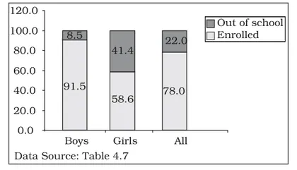
Introduction: "Presentation of Data" is the first practical chapter in Class XI Statistics for Economics. It teaches how raw numerical information is organised and displayed so that patterns, relationships and comparisons become clear. The chapter covers methods for summarising data in tabular, diagrammatic and graphical forms, and the rules and conventions needed to present data correctly and effectively. Importance: Presenting data clearly is essential in economics — for analysing markets, interpreting surveys, reporting class results and supporting arguments. Good presentation makes complex data accessible, helps avoid misinterpretation and supports evidence-based conclusions. Key themes: types of data (qualitative/quantitative, discrete/continuous), frequency distributions and their construction (class limits, class boundaries, class width, class mark), relative and cumulative frequency, methods of tabular presentation (simple and frequency tables), diagrammatic and graphical methods (bar diagrams — simple, multiple, and component; histograms; frequency polygons; ogives/cumulative frequency curves; pie charts; pictograms; line graphs; scatter diagrams), rules and conventions…
Learning Objectives
- Define raw data, attributes, variables, and distinguish between qualitative and quantitative data
- Explain discrete and continuous variables and their implications for data grouping
- Prepare frequency distribution tables for ungrouped and grouped data, choosing appropriate class intervals
- Calculate class boundaries, class marks (mid-points), class widths and cumulative frequencies
- Draw and interpret simple, multiple and sub-divided bar diagrams for categorical data
- Construct pie charts for categorical data and compute central angles from frequencies
- Plot histograms for grouped continuous data and explain the relationship between area and frequency
- Construct frequency polygons and frequency curves from grouped data
Topics in this chapter
8 topics · tap a topic title to jump straight to it.
Introduction to Presentation of Data
What is presentation of data? Presentation of data means arranging collected facts and figures in a systematic, meaningful form so that underlying patterns, trends and relationships become clear and easy to interpret. It converts raw numerical or categorical information into tables, diagrams and graphs.
Why is it important?
- Simplifies complex data and saves time.
- Makes comparison and interpretation easier.
- Helps reveal trends, central tendencies and variability.
- Aids decision-making and communication of findings.
Types of data relevant to presentation
- Qualitative (categorical): e.g., occupation, region, sector. Best shown by bar diagrams and pie charts.
- Quantitative:
- Discrete (countable): e.g., number of children in households. Use frequency tables, bar charts.
- Continuous (measurable): e.g., height, marks, income. Use frequency distribution, histogram, ogive, frequency polygon.
- Primary vs Secondary: Primary data are collected firsthand; secondary are from published sources. Presentation methods are same for both.
Basic steps in presentation
- Classify data (group into classes if continuous or numerous discrete values).
- Construct a frequency distribution (absolute frequencies, relative frequencies, cumulative frequencies).
- Choose appropriate diagram/graph depending on the type of data and purpose.
Key ideas to remember when presenting data
- Label axes, give a clear title, units of measurement and a legend if needed.
- Choose suitable class-widths; avoid too many or too few classes.
- For unequal class widths in a histogram use frequency density (area proportional to frequency).
- Avoid misleading visuals (inaccurate scales, truncated axes, unnecessary 3D effects).
How presentation helps analysis — using tables and graphs you can quickly identify central tendencies (mean/median/mode), spread (range, quartiles) and patterns such as seasonality, growth/decline and concentration.
- Marks of 200 students are grouped into class intervals to form a frequency distribution and represented by a histogram to see the distribution of marks (skewed, symmetric, etc.).
- Population by state is shown with a bar diagram to compare sizes; percentage share of population by sector (agriculture, industry, services) is shown using a pie chart.
- Monthly rainfall for a year is plotted as a line graph to observe seasonal variation and identify wet and dry months.
- Household expenditure categories (food, housing, education, health, transport) displayed as a pie chart to show proportionate spending.
- Class width (approx.) = (Maximum value − Minimum value) / Number of classes
- Class midpoint (xi) = (Lower class limit + Upper class limit) / 2
- Relative frequency = Frequency / Total frequency
- Percentage = Relative frequency × 100
- Cumulative frequency (CF) = Sum of frequencies up to that class
- Frequency density (for unequal class widths) = Frequency / Class width
Types and Classification of Data
Definition: Data are facts, numbers or information collected for reference, analysis and decision making. In economics, data form the basis for statistical analysis and presentation.
Main types of data:
- By source
- Primary data: Collected first-hand for a specific purpose (e.g., survey responses, experiments).
- Secondary data: Collected earlier by someone else (e.g., census reports, published articles).
- By nature (qualitative/quantitative)
- Qualitative (categorical): Non-numeric attributes (e.g., gender, religion, occupation). Subtypes: nominal (no order) and ordinal (with order).
- Quantitative (numerical): Numeric measurements. Subtypes: discrete (countable integers) and continuous (measurable on a continuum).
- By time
- Cross-sectional: Data collected at a single point of time across units (e.g., household consumption in 2023 across states).
- Time-series: Observations on the same variable at successive time points (e.g., GDP each year from 2000–2020).
- By form
- Ungrouped (raw) data: Each observation listed separately (e.g., marks of 30 students).
- Grouped data: Observations organized into class intervals or categories with frequencies (e.g., heights grouped into 150–155 cm, 155–160 cm, ...).
Principles / Rules for classification
- Classes or categories must be mutually exclusive (no overlap).
- They must be collectively exhaustive (cover all observations).
- Classes should be simple and homogeneous and suitable for the purpose of analysis.
- Class intervals are usually of equal width (unless justified otherwise).
Important derived concepts
- Frequency (f): number of observations in a class or category.
- Relative frequency: fraction/ proportion of total: f/N.
- Cumulative frequency: running total of frequencies up to a class.
Why classify? Classification groups data to reveal patterns, simplify analysis and make graphical representation meaningful (e.g., making histograms, ogives, pie charts).
- Primary data: Responses from a household consumption survey conducted this year.
- Secondary data: GDP figures published by the government (annual reports).
- Qualitative nominal: Religion of respondents (Hindu, Muslim, Christian, Other).
- Qualitative ordinal: Education level (Primary, Secondary, Graduate).
- Quantitative discrete: Number of children in each family (0,1,2,3...).
- Quantitative continuous: Heights of students measured in cm (can take any value in an interval).
- Total observations: N = Σ f_i
- Relative frequency: r_i = f_i / N
- Percentage frequency: p_i = (f_i / N) × 100
- \[Cumulative frequency (up to ith class): CF_i = Σ_{j=1}^i f_j\]
- Class width (for k classes): h ≈ (Max − Min) / k
- Class mark (midpoint) of a class: m = (Lower limit + Upper limit) / 2
Tabular Presentation
What is Tabular Presentation?
Tabular presentation is a method of arranging raw data in rows and columns (a table) so that it becomes organised, easy to read and ready for analysis. A well-constructed table summarises data, highlights patterns and supports comparison.
Components of a table
- Title: concise and descriptive.
- Headings/Column titles: name of variables and units of measurement.
- Stub (row labels): labels for rows (e.g., categories or class intervals).
- Body: cells containing the data or frequencies.
- Footnote/Source: any clarifications or data source.
Types of tables
- Simple table: Records individual observations (ungrouped data).
- Frequency distribution table: Groups observations into classes and lists frequencies (grouped data).
- Two-way (contingency) table: Shows joint distribution of two variables (e.g., gender × pass/fail).
Steps / Rules to construct a good table
- Give a clear title and state the period/units.
- Arrange categories logically (chronological, numeric, or alphabetical order).
- Use appropriate class intervals (mutually exclusive, exhaustive, preferably equal width for histograms).
- Include totals (e.g., total frequency).
- Keep layout neat: align numbers (usually right-aligned) and use consistent precision (decimal places).
Advantages and limitations
- Advantages: simplifies large data sets, reveals patterns, makes comparison easier, is a basis for graphical presentation.
- Limitations: grouping causes loss of individual detail; poor choice of classes can hide information.
Small example table (marks of 10 students)
| Student | Marks |
|---|---|
| A | 78 |
| B | 62 |
| C | 85 |
Example: Frequency distribution (grouped)
| Marks (class) | Frequency (f) |
|---|---|
| 0–10 | 1 |
| 11–20 | 3 |
| 21–30 | 5 |
| 31–40 | 1 |
Such tables are the starting point for graphs like histograms, frequency polygons and ogives.
- Monthly household expenditure table: categories (Food, Rent, Education, Transport) with amounts for each month.
- Attendance record of students: dates as columns and student names as rows, marking presence/absence.
- Marks distribution of a class presented as a frequency table with class intervals (0–9, 10–19, ... ) and corresponding frequencies.
- Population by age groups in a city: age intervals (0–14, 15–24, 25–44, …) and number of persons in each group.
- Two-way table: number of males and females who passed/failed an exam (gender × result).
- Total frequency: N = Σ fi
- Relative frequency of class i: ri = fi / N
- Percent frequency: pi = (fi / N) × 100
- Class width (approx.): h ≈ (Range) / (Number of classes) where Range = Max − Min (round up if needed)
- Class midpoint (xi): xi = (Lower limit + Upper limit) / 2
- Cumulative frequency (up to class k): CFk = Σ (fi) for i = 1 to k
Diagrammatic Methods
What are Diagrammatic Methods?
Diagrammatic methods are graphical techniques used to present statistical data visually so patterns, trends and comparisons become easier to understand. They convert numerical tables into charts or diagrams (bars, pie, histograms, polygons, ogives, line graphs, pictograms) that communicate information quickly.
Why use them?
- Make large data sets easier to interpret.
- Highlight trends, comparisons and composition at a glance.
- Useful for report writing, presentations and decision making.
General rules for good diagrams
- Choose the diagram that suits the data and purpose (comparison, composition, distribution or time series).
- Label axes, units and categories clearly; give a title and source.
- Use uniform scale; avoid 3D effects that distort perception.
- Provide a legend if there are multiple series or symbols.
- If using pictograms, state the value represented by one symbol.
Common diagram types and how to prepare them
1. Bar Diagram — used for comparing discrete categories (e.g., sales by state)
- Axes: categories on x-axis, frequency/value on y-axis.
- Bars should be of equal width and equidistant (vertical or horizontal).
- Variations: simple, multiple (grouped) bars for comparing sub-groups, and component (stacked) bars to show parts of a whole.
2. Pie Diagram (Pie Chart) — shows composition (parts of a whole)
- Convert each category to an angle: Angle = (Category value / Total) × 360°.
- Draw slices proportionally; include labels or a legend with percentages.
3. Histogram — for continuous data grouped into class intervals (e.g., income, age)
- Plot class intervals on x-axis and frequency on y-axis as adjacent rectangles (no gaps).
- If class widths are unequal, use frequency density = frequency / class width for heights.
4. Frequency Polygon — alternative to histogram to show distribution shape
- Use class mid-points on x-axis and plot frequencies as points; join points with straight lines.
- Extend polygon to the x-axis at ends (by adding a class with zero frequency) to close the shape.
5. Ogive (Cumulative Frequency Curve) — shows cumulative frequencies and is useful for median/percentile estimation
- Plot cumulative frequency against upper class boundaries (or lower boundaries) and join points with a smooth curve or straight lines.
6. Line Graph (Time Series) — shows trends over time (months, years)
- Plot time on x-axis and variable on y-axis; mark data points and join with straight lines.
7. Pictogram — uses pictures/icons to represent quantities (good for simple public displays)
- One symbol must represent a fixed quantity; include a key (e.g., 1 icon = 100 students).
Advantages
- Quick visual impression, easier comparison and interpretation.
- Can reveal patterns (trend, seasonal effects, skewness) not obvious in tables.
Limitations
- Poorly drawn diagrams can mislead (incorrect scales, truncated axes, 3D effects).
- Not suitable for very detailed numerical analysis; best for summary presentation.
Practical steps when preparing a diagram
- Decide the objective (compare categories, show composition, show distribution or trend).
- Choose the appropriate diagram type.
- Compute necessary derived values (percentages, angles, midpoints, frequency densities, cumulative frequencies).
- Draw axes, mark scale carefully and plot; label everything and add a title and source.
- Pie chart: A company’s market share in a year — convert each company’s sales to percentage of total and plot slices (Angle = (sales/total sales) × 360°).
- Bar diagram: Compare annual revenues of 4 states — use vertical bars with states on x-axis and revenue on y-axis to compare magnitudes.
- Histogram: Distribution of students’ marks grouped in class intervals (0–10, 10–20, …). If class widths are equal, plot frequencies as adjacent bars; if unequal, use frequency density.
- Frequency polygon: Show the shape of the marks distribution by plotting mid-points of intervals (e.g., 5, 15, 25…) against frequencies and joining with lines.
- Ogive: To find median marks from grouped data, plot cumulative frequency against upper class boundaries and read off the median (N/2) on y-axis, then project to x-axis.
- Line graph: Monthly sales over a year — months on x-axis, sales on y-axis; connect points to show trend and seasonality.
- Angle for pie chart = (Category value / Total) × 360°
- Percentage of total = (Category value / Total) × 100
- Class midpoint (xᵢ) = (Lower class boundary + Upper class boundary) / 2
- Class width (h) = Upper limit − Lower limit
- Frequency density (for unequal class widths) = Frequency / Class width
- Cumulative frequency (cf) = Σ frequencies up to that class
Graphical Methods
Graphical methods are visual techniques used to present statistical data so patterns, trends, comparisons and distributions become easy to understand. They convert numbers into pictures (bars, lines, circles, polygons, etc.), which help in quick interpretation and communication.
Key principles when drawing any graph:
- Choose the appropriate type of graph for the data (categorical, discrete, continuous, time-series, bivariate).
- Label axes with variable names and units, give a clear title, and include a legend if needed.
- Select a suitable scale so the entire data range fits and the graph is not distorted.
- Use class boundaries (continuous scale) for histograms and ogives, and mid-points for frequency polygons.
Main graphical methods:
- Bar Diagram — Simple bars for categorical or discrete data. Bars are separated by gaps. Variants: multiple bar (two or more series side-by-side) and sub-divided/stacked bar (components stacked within a single bar).
- Pie Chart — Circle divided into sectors showing proportional composition. Useful for parts of a whole.
- Histogram — Used for continuous grouped data. Adjacent bars with no gaps. Height represents frequency density when class widths differ.
- Frequency Polygon — Points plotted at class mid-points with ordinate equal to frequency (or frequency density) and joined by straight lines. Useful for comparing distributions.
- Ogive (Cumulative Frequency Curve) — Plots cumulative frequency against class boundaries. Two types: "less than" ogive and "more than" ogive. Intersection gives median and quartiles.
- Line Graph (Time Series) — Points for observations over time joined by lines. Ideal for showing trends.
- Scatter Plot — Plots paired (x,y) data to show relationship or correlation between two variables.
- Pareto Chart — Bars in descending order of frequency and a cumulative percentage line; highlights the most important factors (80/20 rule).
Interpretation tips:
- Shape of distribution (symmetric, positively/negatively skewed) can be seen from histograms and frequency polygons.
- Ogive helps locate median (point where cumulative frequency = N/2) and quartiles (N/4, 3N/4).
- Scatter plots indicate direction and strength of relationship; add a trend line to see correlation.
- Population by religion in a state — use a pie chart to show percentage share of each religion.
- Monthly sales of a shop over a year — use a line graph (time-series) to show trends and seasonality.
- Marks obtained by students grouped into classes (40–49, 50–59, ...) — use a histogram to show distribution of marks and a frequency polygon to compare with another class.
- Number of households having different income ranges — use a bar diagram for distinct income brackets or a histogram if income is treated continuous.
- Height and weight of individuals — use a scatter plot to examine correlation between height (x-axis) and weight (y-axis).
- Causes of machine breakdowns ranked by frequency — use a Pareto chart to identify the most frequent causes and cumulative percent line to apply the 80/20 principle.
- Class midpoint (xi) = (lower class boundary + upper class boundary) / 2
- Class width (h) = upper limit - lower limit (or upper boundary - lower boundary)
- Frequency density (for histogram) = frequency (fi) / class width (h)
- Angle for pie chart (in degrees) = (fi / Σfi) × 360
- Percentage for a category = (fi / Σfi) × 100
- Cumulative frequency (CF) at a class = sum of frequencies up to that class
Construction Steps and Conventions
Overview
"Construction Steps and Conventions" describes how to convert raw data into classed frequency tables and graphical displays (histogram, frequency polygon, ogive, bar chart, pie chart etc.) using standard steps and rules so graphs are accurate, comparable and not misleading.
- Collect and sort data
Obtain the raw data and arrange it in ascending order (if individual values) or prepare an initial tally. - Decide number of classes (k)
Use judgment or a rule (e.g. Sturges' rule: k ≈ 1 + 3.322 log10 n). Typical k is between 5 and 15 depending on sample size. - Compute range and class width
Range = max − min. Class width (h) ≈ Range / k. Round h to a convenient number (1, 2, 5, 10 …) so classes are simple. - Form class intervals
Choose a suitable starting point and make k non-overlapping intervals of equal width (unless unequal widths are needed). Write class limits (e.g. 10–19, 20–29). - Convert to class boundaries (for continuous presentation)
For continuous graphs (histograms, ogives) use class boundaries so adjacent classes touch. If original classes were 10–19 and 20–29 (discrete limits), boundaries become 9.5–19.5 and 19.5–29.5 (subtract/add half the measuring unit). - Tabulate frequencies
Count observations in each class → frequency (f). Also compute cumulative frequency (CF), relative frequency (f/N) and percentage frequency. - Adjust for unequal class widths
If class widths differ, use frequency density = frequency / class width on the vertical axis for histograms so area represents frequency. - Choose representation and draw
- Decide histogram, frequency polygon, ogive, bar chart, pie chart, line graph or Pareto chart.
- Draw axes, choose an appropriate scale (use simple numbers; ensure axis for bar/hist starts at zero), plot points/rectangles/angles, join where needed, add title, labels, legend and source.
- Conventions to follow
- Bars touch in histograms (continuous data); bars separated in bar charts (discrete categories).
- Use class boundaries for histograms and ogives; use class marks (mid‑points) for frequency polygons.
- Vertical axis normally starts at zero for bar/histogram to avoid misleading visual effects.
- When class widths unequal, plot frequency density (height) so area ∝ frequency.
- Label axes clearly (variable and units), give a descriptive title and provide source of data.
How it looks in practice (short workflow): Raw data → choose k and h → create class intervals and boundaries → tally frequencies → compute CF/relative frequencies/frequency density (if needed) → choose chart → draw axes with scale → plot and label.
- Example 1 (Histogram): Marks of 40 students range from 12 to 92. Range = 80. Choose k = 8, class width h = 10. Classes: 10–19, 20–29, …, 80–89, 90–99. Compute frequency for each class, use class boundaries (9.5–19.5 etc.) and draw touching bars with heights equal to frequencies. Title: 'Distribution of Marks — 40 Students'.
- Example 2 (Unequal class widths): Suppose time spent on a website (mins) grouped as 0–5, 5–15, 15–60 with frequencies 50, 30, 20. Class widths are 5, 10, 45. Compute frequency density = f / width → 10, 3, 0.444. For histogram plot heights = frequency densities; area (width × height) of each bar equals the class frequency, preserving correct visual weight.
- Example 3 (Ogive): For the marks example, compute cumulative frequencies up to each upper class boundary (e.g. ≤19, ≤29 …). Plot CF on vertical axis against class boundaries on horizontal axis and join points to form the ogive. The ogive helps read median and percentiles by interpolation.
- Range = Maximum value − Minimum value
- Sturges' rule (approx.) for number of classes: k ≈ 1 + 3.322 log10(n)
- Class width h ≈ Range / k (round to a convenient value)
- Class mark (mid‑point) m = (Lower limit + Upper limit) / 2
- Class boundary (continuous) for limit a–b: lower boundary = a − 0.5×(unit), upper boundary = b + 0.5×(unit) (use appropriate unit of measurement)
- Cumulative frequency (CF) for jth class = Σ (frequencies up to jth class)
Interpretation and Analysis
Definition: Interpretation means explaining what the presented data shows (patterns, direction, comparisons). Analysis goes further: it examines causes, relationships, reliability and implications of the data and suggests conclusions or actions.
Purpose: To convert numbers into meaningful information for decision-making — e.g., identifying trends, comparing groups, detecting outliers, and testing relationships.
Step-by-step approach
- Understand the data: units, period, population/sample, base (for index numbers) and any missing values.
- Summarise appropriately: use totals, averages, percentages, rates, or index numbers depending on the question.
- Visualise: choose a graph that matches the aim (trend, composition, distribution, relationship).
- Compute measures: central tendency (mean/median/mode), dispersion (range, standard deviation, coefficient of variation), growth rates or index numbers as needed.
- Interpret patterns: direction (increasing/decreasing), seasonality, peaks/troughs, anomalies/outliers and relative comparisons (use percentages or per-capita measures for fair comparison).
- Analyse causes and implications: relate observed patterns to possible economic, social or policy factors and assess reliability (sample size, data quality, scale or aggregation bias).
- Conclude with clear, evidence-based statements and, if required, recommendations.
Common pitfalls to watch for
- Misleading scales or truncated axes in graphs.
- Confusing absolute values with relative change — use percent change for comparison over time or across sizes.
- Aggregating heterogeneous groups without standardisation (per capita or rates may be needed).
- Ignoring outliers or small sample sizes when generalising.
How interpretation and analysis are used in economics
- Policymakers read time-series data (GDP, inflation) to decide fiscal or monetary measures.
- Firms analyse sales trends and seasonality to plan production and inventory.
- Researchers use scatter plots and regression to test relationships (e.g., income vs consumption).
- Year-to-year GDP growth: compute percent change in GDP, draw a time-series line graph, add a trend line or moving average to identify long-term growth vs short-term fluctuations, then discuss possible causes (investment, exports, policy changes).
- School marks distribution: calculate mean, median, mode and standard deviation; draw a histogram and box plot to identify spread and outliers; interpret whether most students cluster around a central score or scores vary widely.
- Monthly household budget: convert absolute spending to percentages of total expenditure and present a pie chart to interpret composition (food, housing, education); analyse which category dominates and suggest areas to cut spending.
- Commodity prices and inflation: construct index numbers (base year = 100) for price series, compare real vs nominal changes, and interpret how inflation affects purchasing power.
- Rainfall and crop yield: use a scatter plot of annual rainfall (x) vs yield (y), fit a trend/regression line to analyse relationship and test whether higher rainfall is associated with higher yield or whether other factors matter.
- Arithmetic mean (ungrouped): x̄ = Σx / n, where Σx = sum of observations, n = number of observations.
- Arithmetic mean (grouped): x̄ = Σ(f * m) / N, where f = class frequency, m = class midpoint, N = Σf.
- Median (grouped): Median = L + ((N/2 - c.f.) / f) * h, where L = lower class boundary of median class, c.f. = cumulative frequency before median class, f = frequency of median class, h = class width, N = total frequency.
- Mode (grouped): Mode = L + (d1 / (d1 + d2)) * h, where d1 = f1 - f0, d2 = f1 - f2, f1 = frequency of modal class, f0 = frequency of previous class, f2 = frequency of next class, h = class width.
- Standard deviation (population): σ = sqrt(Σ(x - x̄)^2 / N). (For a sample use denominator n-1.)
- Coefficient of variation: CV (%) = (σ / x̄) * 100 — useful for comparing relative variability of different series.
Practical Applications and Exercises
What this topic covers: Practical Applications and Exercises in "Presentation of Data" teaches how to convert raw observations into organised tables and graphs that make patterns visible and support interpretation. You learn to form frequency distributions, compute relative and cumulative frequencies, choose suitable graphical forms (bar chart, histogram, frequency polygon, ogive, pie chart, time-series line), and interpret results to draw conclusions.
Step-by-step practical procedure:
- Collect and inspect raw data: Check for measurement units, discrete vs continuous nature, and any obvious errors/outliers.
- Decide grouping: For large/raw numeric data, form class intervals. Prefer 5–15 classes depending on sample size. Use equal class width if possible.
- Compute class boundaries and mid-points: Convert limits to continuous class boundaries (adjust by half the smallest measurement unit, commonly 0.5 when units are whole numbers). Mid-point = (lower limit + upper limit)/2.
- Build frequency table: Tally frequencies, then compute relative frequencies (f / N), cumulative frequencies, and frequency density if class widths vary (frequency density = f / class width).
- Choose the right visual form: Qualitative/discrete—bar chart or pie chart. Continuous—histogram (for frequency), frequency polygon (mid-points joined), ogive (cumulative frequency). Time-series—line graph.
- Draw carefully: Label axes, give a title, choose an appropriate scale, and for histograms use contiguous bars (no gaps). For unequal widths use frequency density on vertical axis.
- Interpret and conclude: Look for central tendency, spread, skewness, modes, peaks, clusters, gaps, and trends over time. Relate findings to the context (e.g., policy implication, business decision).
Exam & classroom tips:
- Always show class limits, boundaries, mid-points and formula steps when asked. Marks are awarded for method and presentation.
- When class widths are unequal, use frequency density for histograms; otherwise heights will mislead.
- To find median or mode from grouped data, use the standard grouped-data formulae (show each symbol and substitution clearly).
- Use ogive to locate median graphically: the median corresponds to cumulative frequency = N/2 on the vertical axis.
Common practical exercises students should practice: constructing frequency distributions, drawing histograms, frequency polygons and ogives, converting a bar chart to a pie chart (percentages), finding mean/median/mode from grouped frequency tables, and interpreting graphs in context.
- Marks of 200 students grouped into class intervals (0–9, 10–19, ...). Create a frequency table, draw a histogram and frequency polygon, compute mean, median and mode from the grouped data, and comment on performance (skewness, modal class).
- Monthly sales (in ₹ thousands) of a shop for two years: present as a time-series line graph, identify seasonal peaks and growth trend, and compute percentage change year-on-year.
- Household income distribution in a locality: construct a grouped frequency table, draw a pie chart showing income-share bands, and use an ogive to estimate the median income.
- Customer wait times (in minutes) recorded at a clinic: form a frequency distribution with equal-width classes, draw a histogram (bars touching), and comment on central tendency and variability.
- Market shares of five companies: present as a pie chart (percentages) and a side-by-side bar chart to compare absolute values across two years.
- Class mid-point (x): x = (lower limit + upper limit) / 2
- Frequency (f), Relative frequency = f / N, where N = Σf
- Cumulative frequency: cumulative total of frequencies up to a class
- Mean for grouped data (direct): Mean = Σ(f × x) / Σf, where x = class mid-point
- Mean by assumed-mean method: Mean = a + [Σ(f × u) / Σf] × h, where u = (x - a)/h, a = assumed mean (mid-point), h = class width
- Median (grouped): Median = l + [(N/2 − cf) / f_m] × h, where l = lower class boundary of median class, cf = cumulative frequency before median class, f_m = frequency of median class, h = class width
Key Concepts
- Data
- Facts, numbers or information collected for analysis or decision making.
- Primary data
- Data collected firsthand by the researcher for a specific purpose.
- Secondary data
- Data that have been collected earlier by someone else and reused.
- Frequency distribution
- Organization of raw data into classes or categories with their corresponding frequencies.
- Class interval
- A range of values that forms one group in a frequency distribution.
- Class width (class size)
- The difference between the upper and lower limits of a class interval.
- Class limits
- The smallest and largest values that can belong to a class (lower limit and upper limit).
- Inclusive and exclusive class limits
- Inclusive limits include both end values; exclusive limits include the lower but exclude the upper value.
- Class boundaries
- Values that remove gaps between successive classes, usually obtained by adding/subtracting 0.5 when data are whole numbers.
- Class mark (midpoint)
- The value halfway between the lower and upper class limits; (lower limit + upper limit)/2.
- Frequency
- The number of observations falling in a particular class or category.
- Cumulative frequency
- The running total of frequencies up to a given class or category.
- Relative frequency
- The proportion of the total observations that lie in a class; frequency divided by total frequency.
- Percentage frequency
- Relative frequency expressed as a percentage (relative frequency × 100).
- Histogram
- A graphical representation of a frequency distribution using contiguous bars whose heights represent frequencies.
- Frequency polygon
- A line graph formed by joining midpoints of class intervals plotted against their frequencies.
- Ogive
- A cumulative frequency curve showing 'less than' or 'more than' cumulative frequencies against class boundaries.
- Bar graph (bar diagram)
- A chart using separate rectangular bars with equal width and gaps to compare discrete categories or values.
- Pie chart (circle graph)
- A circular chart divided into sectors where each sector’s angle/area represents a category’s proportion of the total.
- Pictogram (pictograph)
- A diagram that uses pictures or symbols to represent data where each symbol stands for a specified number of units.
End-of-Chapter Trial Paper & Test Questions
Topic-wise questions to test your understanding of every concept in this chapter.
-
Distinguish between qualitative and quantitative data, giving one example of each and the most suitable diagram for it. / गुणात्मक और मात्रात्मक आँकड़ों में अंतर बताइए, प्रत्येक का एक उदाहरण तथा उसके लिए सर्वाधिक उपयुक्त आरेख दीजिए।
Show answer
Qualitative (categorical) data describe non-numeric attributes such as occupation or religion and are best shown by bar diagrams or pie charts. Quantitative data are numeric, such as height or income, and continuous quantitative data are best shown by a histogram. / गुणात्मक (श्रेणीगत) आँकड़े व्यवसाय या धर्म जैसी गैर-संख्यात्मक विशेषताएँ बताते हैं और दंड आरेख या वृत्त आरेख से सर्वोत्तम दर्शाए जाते हैं। मात्रात्मक आँकड़े संख्यात्मक होते हैं, जैसे ऊँचाई या आय, और सतत मात्रात्मक आँकड़े आयतचित्र (हिस्टोग्राम) से सर्वोत्तम दर्शाए जाते हैं।
-
Differentiate between class limits and class boundaries, and convert the inclusive class 10–19 (whole-number data) into class boundaries. / वर्ग सीमाओं और वर्ग परिसीमाओं में अंतर कीजिए, तथा समावेशी वर्ग 10–19 (पूर्ण-संख्या आँकड़े) को वर्ग परिसीमाओं में बदलिए।
Show answer
Class limits are the smallest and largest values that can belong to a class, while class boundaries remove the gap between successive classes (used for histograms/ogives). For 10–19 with whole-number data, subtract and add 0.5 to get boundaries 9.5–19.5. / वर्ग सीमाएँ वे न्यूनतम व अधिकतम मान हैं जो किसी वर्ग में हो सकते हैं, जबकि वर्ग परिसीमाएँ क्रमागत वर्गों के बीच का अंतर हटाती हैं (आयतचित्र/तोरण हेतु)। 10–19 के लिए पूर्ण-संख्या आँकड़ों में 0.5 घटाकर व जोड़कर परिसीमाएँ 9.5–19.5 प्राप्त होती हैं।
-
Household expenditure on food is ₹3,000 out of a total monthly budget of ₹12,000. Compute the central angle for 'food' in a pie chart. / मासिक बजट ₹12,000 में से भोजन पर घरेलू व्यय ₹3,000 है। वृत्त आरेख में 'भोजन' का केंद्रीय कोण ज्ञात कीजिए।
Show answer
Angle = (category value / total) × 360° = (3000/12000) × 360° = 0.25 × 360° = 90°. / कोण = (श्रेणी मान / कुल) × 360° = (3000/12000) × 360° = 0.25 × 360° = 90°।
-
Why must the heights of a histogram represent frequency density rather than frequency when class widths are unequal? / जब वर्ग चौड़ाइयाँ असमान हों तो आयतचित्र की ऊँचाइयाँ आवृत्ति के बजाय आवृत्ति घनत्व क्यों दर्शानी चाहिए?
Show answer
In a histogram the area of each bar must be proportional to the frequency. With unequal class widths, using raw frequency as height distorts areas, so frequency density (frequency ÷ class width) is used so that area = width × density correctly represents the class frequency. / आयतचित्र में प्रत्येक दंड का क्षेत्रफल आवृत्ति के समानुपाती होना चाहिए। असमान वर्ग चौड़ाइयों में ऊँचाई के रूप में कच्ची आवृत्ति प्रयोग करने से क्षेत्रफल विकृत हो जाता है, अतः आवृत्ति घनत्व (आवृत्ति ÷ वर्ग चौड़ाई) प्रयोग किया जाता है ताकि क्षेत्रफल = चौड़ाई × घनत्व वर्ग आवृत्ति को सही दर्शाए।
-
How does a histogram differ from a bar diagram in construction? / निर्माण की दृष्टि से आयतचित्र दंड आरेख से किस प्रकार भिन्न है?
Show answer
In a histogram the bars are adjacent and touch each other because data are continuous and class intervals are contiguous, whereas in a bar diagram the bars have equal width but are separated by gaps because the data are discrete or categorical. / आयतचित्र में दंड एक-दूसरे से सटे (स्पर्श करते) होते हैं क्योंकि आँकड़े सतत होते हैं और वर्ग-अंतराल लगातार होते हैं, जबकि दंड आरेख में दंड समान चौड़ाई के होते हैं पर अंतराल से अलग रहते हैं क्योंकि आँकड़े विविक्त या श्रेणीगत होते हैं।
-
Marks of 40 students range from 12 to 92. Using Sturges' rule guidance, find the range and a convenient class width if 8 classes are chosen. / 40 विद्यार्थियों के अंक 12 से 92 तक हैं। यदि 8 वर्ग चुने जाएं तो परास तथा एक सुविधाजनक वर्ग चौड़ाई ज्ञात कीजिए।
Show answer
Range = Maximum − Minimum = 92 − 12 = 80. Class width h ≈ Range/k = 80/8 = 10, which is already a convenient round number, so h = 10. / परास = अधिकतम − न्यूनतम = 92 − 12 = 80। वर्ग चौड़ाई h ≈ परास/k = 80/8 = 10, जो पहले से ही सुविधाजनक पूर्ण संख्या है, अतः h = 10।
-
What is an ogive and how is it used to read the median? / तोरण (ओजाइव) क्या है और इसका उपयोग माध्यिका पढ़ने के लिए कैसे किया जाता है?
Show answer
An ogive is a cumulative frequency curve plotting cumulative frequency against class boundaries. To read the median, mark N/2 on the cumulative-frequency (y) axis, draw a horizontal line to the curve, and drop a perpendicular to the x-axis; the x-value gives the median. / तोरण एक संचयी आवृत्ति वक्र है जो संचयी आवृत्ति को वर्ग परिसीमाओं के सापेक्ष आलेखित करता है। माध्यिका पढ़ने हेतु संचयी-आवृत्ति (y) अक्ष पर N/2 अंकित करें, वक्र तक क्षैतिज रेखा खींचें और x-अक्ष पर लंब डालें; वह x-मान माध्यिका देता है।
-
List two common ways in which a graph can mislead the reader. / दो सामान्य तरीके बताइए जिनसे कोई आरेख पाठक को भ्रमित कर सकता है।
Show answer
Two ways are: using inaccurate or truncated axis scales (e.g., a y-axis not starting at zero, exaggerating differences), and using unnecessary 3D effects or distorted symbols that misrepresent relative magnitudes. / दो तरीके हैं: गलत या कटी-छँटी अक्ष-मापनी का प्रयोग (जैसे y-अक्ष का शून्य से न शुरू होना, जिससे अंतर बढ़े-चढ़े दिखें), तथा अनावश्यक त्रिविमीय (3D) प्रभाव या विकृत प्रतीकों का प्रयोग जो सापेक्ष परिमाण को गलत दर्शाते हैं।
Related Laws & Principles
Explore allFoundational laws & principles behind this chapter. Each one opens a full page — what it says, why it matters, five practice questions and the mistakes to avoid.