Overview
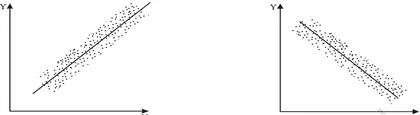
Introduction: Correlation is a statistical tool that measures the degree and direction of association between two quantitative variables. In the CBSE Class 11 Economics chapter "Correlation" (Statistics for Economics), students learn how to identify, measure and interpret relationships between economic variables — for example, income and expenditure, price and demand, or savings and investment. Importance: Understanding correlation helps students describe economic relationships, summarize bivariate data, and make informed interpretations of how two variables move together. It is a foundation for further study of regression and for empirical analysis in economics, where recognizing associations is essential before exploring causation. Key themes covered: - Graphical representation using scatter (scatter) diagrams to visualize the direction and form of association. - Types of correlation: positive, negative (inverse), and zero (no correlation), and special cases of perfect correlation. - Measures of correlation: Karl Pearson's coefficient of correlation (product-moment method) for measuring linear association and Spearman's rank correlation coefficient for ordinal or ranked data. -…
Learning Objectives
- Define correlation and correlation coefficient for bivariate data.
- Explain different types of correlation (positive, negative, zero and negligible) with economic examples.
- Distinguish between correlation and causation in economic relationships.
- Describe the construction and interpretation of a scatter diagram to detect correlation.
- Draw a scatter diagram for given paired observations and comment on the nature of correlation.
- Compute Karl Pearson's coefficient of correlation from raw ungrouped data.
- Calculate Karl Pearson's coefficient of correlation from grouped (frequency) data.
- Apply Spearman's rank correlation coefficient to analyze ordinal or ranked data.
Topics in this chapter
12 topics · tap a topic title to jump straight to it.
Meaning and Definition of Correlation
Meaning: Correlation is a statistical measure that describes the direction and degree of association between two variables. It tells us whether and how strongly two variables move together.
Definition (simple): Correlation between two variables exists if values of one variable are related systematically to values of the other. In economics, correlation helps to study relationships such as price and demand, income and consumption, or advertising and sales.
Formal idea: If high (or low) values of X are associated with high (or low) values of Y, X and Y are positively correlated. If high values of X are associated with low values of Y, they are negatively correlated. If no systematic relationship is observed, there is zero (or no) correlation.
Key characteristics:
- Direction: positive, negative, or zero.
- Degree (strength): ranges from weak to strong; measured numerically by correlation coefficients (e.g., Pearson's r, Spearman's rho).
- Unit-free: correlation coefficients do not depend on the units of measurement.
- Correlation does not imply causation: a statistical association does not prove one variable causes the other.
Types of correlation:
- Perfect positive correlation: all points lie on an upward straight line (coefficient = +1).
- Perfect negative correlation: all points lie on a downward straight line (coefficient = −1).
- Imperfect (partial) correlation: points form a cloud with a clear trend upward or downward (|r| < 1).
- No correlation: points show no discernible pattern (r ≈ 0).
- Linear vs. non-linear (curvilinear) correlation: association may be roughly straight-line or curved.
How it is studied: The simplest graphical method is a scatter diagram (scatter plot) where each pair (x_i, y_i) is plotted. Numerical measures include covariance and correlation coefficients (Pearson's r for linear association; Spearman's rho for ranks).
Why it is useful in economics: Correlation helps to identify relationships for forecasting, policy analysis and decision making — for example, how income changes with education, or how demand changes with price. But economists must test causality separately (experiments, instrumental variables, time series analysis).
- Study hours and exam marks: usually a positive correlation — more study hours are associated with higher marks.
- Price of a commodity and quantity demanded: typically a negative correlation — as price rises, quantity demanded falls (ceteris paribus).
- Advertising expenditure and sales: often a positive correlation — higher advertising is associated with higher sales.
- Distance from city center and rent: generally negative correlation — rents fall as distance from centre increases.
- Temperature and sale of ice-cream: positive correlation — higher temperature tends to increase ice-cream sales.
- Covariance: Cov(X,Y) = (1/n) Σ (x_i - x̄)(y_i - ȳ) — indicates direction of linear relationship (positive or negative).
- Pearson's coefficient of correlation (population form): r = [Σ (x_i - x̄)(y_i - ȳ)] / sqrt([Σ (x_i - x̄)^2] [Σ (y_i - ȳ)^2]) — ranges from −1 to +1; measures strength and direction of linear association.
- Interpretation of r: r = +1 (perfect positive), r = −1 (perfect negative), r = 0 (no linear correlation).
- Spearman's rank correlation (for ordinal/ranked data): ρ = 1 − (6 Σ d_i^2) / [n(n^2 − 1)], where d_i = difference in ranks for pair i.
Types of Correlation
Definition: Correlation describes the degree and direction of association between two quantitative variables. It does not imply causation — only how two variables move together.
Main types of correlation:
- Positive (Direct) correlation: As one variable increases, the other also increases. Points on a scatter plot trend upward from left to right. Degree can be perfect, high, moderate or low.
- Negative (Inverse) correlation: As one variable increases, the other decreases. Points trend downward from left to right. Degree can vary from perfect to weak.
- No (Zero) correlation: No discernible pattern; variables do not show any consistent increase or decrease together.
- Perfect correlation: All points lie exactly on a straight line. Pearson correlation coefficient r = +1 (perfect positive) or r = −1 (perfect negative).
- Imperfect/Partial correlation: Points roughly follow a trend but are scattered around a line (common in real data). Degree described as high, moderate or low.
- Linear vs Curvilinear (nonlinear) correlation: Linear correlation follows (approximately) a straight-line relationship. Curvilinear correlation shows a systematic but non‑linear pattern (e.g., U-shaped or inverted-U).
Important point: Correlation coefficient (r) quantifies the direction and strength: r ranges from −1 to +1. The sign gives direction; the magnitude gives strength (|r| close to 1 = stronger linear relationship).
- Positive correlation: Hours of study and marks scored (generally more study → higher marks).
- Negative correlation: Price of a normal good and quantity demanded (higher price → lower demand).
- No correlation: Shoe size and intelligence (no systematic relationship).
- Perfect positive correlation: Temperature measured in Celsius and in Kelvin shifted by a constant when plotted as deviation from a baseline (if scaled appropriately, points lie on a straight line).
- Curvilinear correlation: Age and income—income rises with age up to a point then falls (inverted-U pattern).
- High but not perfect: Advertising expenditure and sales — more ad spending tends to increase sales but other factors cause scatter.
- Pearson's correlation coefficient (sample form): r = Σ(x - x̄)(y - ȳ) / √[Σ(x - x̄)² · Σ(y - ȳ)²]
- Alternate computation (raw scores): r = [nΣxy − (Σx)(Σy)] / √{[nΣx² − (Σx)²] · [nΣy² − (Σy)²]}
- Covariance: Cov(X,Y) = Σ(x - x̄)(y - ȳ) / n (population) or divide by (n−1) for sample covariance)
- Spearman's rank correlation (for ranks): r_s = 1 − [6 Σd²] / [n(n² − 1)], where d = difference between paired ranks
- Interpretation range: −1 ≤ r ≤ +1. Values close to 0 indicate weak/no linear correlation; values near ±1 indicate strong linear correlation.
Scatter Diagram (Scatter Plot)
Definition: A scatter diagram (scatter plot) is a two-dimensional graph used to display paired observations (x, y) so that the relationship between two quantitative variables can be seen visually. Each pair is plotted as a point with horizontal coordinate x and vertical coordinate y.
Purpose: To detect the existence, direction and approximate strength of a relationship (correlation) between two variables before calculating a correlation coefficient or fitting a regression line.
Construction (step-by-step):
- Select the two variables to examine (independent on x-axis, dependent on y-axis).
- Choose suitable scales and label axes with units.
- Plot each paired observation (x, y) as a point.
- Look for a pattern: upward, downward, or no clear pattern.
- If needed, draw a line of best fit (trend line) — often the least squares regression line — and mark the mean point (x̄, ȳ).
Interpretation of patterns:
- Positive correlation: points tend to slope upward from left to right (as x increases, y tends to increase).
- Negative correlation: points slope downward (as x increases, y tends to decrease).
- No correlation: points are scattered randomly with no clear trend.
- Perfect correlation: all points lie exactly on a straight line (rare in real data).
Relation to quantitative measures: A scatter diagram gives a graphical impression of the relationship which is then quantified by the correlation coefficient (r) and by regression equations (y = a + bx).
Uses in Economics (Class 11 context): To visualise relationships such as consumption vs income, advertising expenditure vs sales, price vs quantity demanded (negative relationship), investment vs interest rate, GDP vs employment, etc. It helps in preliminary analysis before formal correlation/regression calculations.
Advantages: Simple, intuitive, shows outliers and non-linear patterns, useful for preliminary analysis.
Limitations: Does not give a numerical measure of strength (need r), may be affected by scale and outliers, visual impression can be subjective.
- Study hours (x) and exam marks (y): plot students' hours studied against marks to see if more study generally leads to higher marks (expected positive correlation).
- Advertising expenditure (x) and monthly sales (y): plot ad spend and sales to visualise whether higher advertising is associated with higher sales (positive correlation).
- Price of a commodity (x) and quantity demanded (y): plot price against quantity demanded to observe the expected negative correlation (demand curve tendency).
- Interest rate (x) and investment (y): plot prevailing interest rates and level of investment to check for a negative relationship (higher rates, lower investment).
- Household income (x) and consumption expenditure (y): plot pairs to examine the income–consumption relationship (positive correlation).
- Pearson correlation coefficient (raw sums): r = [nΣxy − (Σx)(Σy)] / sqrt( [nΣx^2 − (Σx)^2] [nΣy^2 − (Σy)^2] )
- Pearson correlation coefficient (deviation form): r = Σ(x − x̄)(y − ȳ) / sqrt( Σ(x − x̄)^2 · Σ(y − ȳ)^2 )
- Regression line of y on x: y = a + bx, where b = r · (Sy / Sx) and a = ȳ − b·x̄ (Sx, Sy are standard deviations of x and y respectively)
- Interpretation rule of r: −1 ≤ r ≤ 1. r > 0 indicates positive association, r < 0 indicates negative association, |r| near 1 indicates strong linear relationship, |r| near 0 indicates weak linear relationship.
Karl Pearson's Coefficient of Correlation (r)
Definition: Karl Pearson's coefficient of correlation (r) measures the strength and direction of the linear relationship between two continuous variables X and Y. Its value lies between -1 and +1. A positive r indicates that as X increases, Y tends to increase; a negative r indicates that as X increases, Y tends to decrease; r = 0 indicates no linear association.
Mathematical meaning: For a sample of n paired observations (x_i, y_i), Pearson's r is the standardized covariance of X and Y. It quantifies how much X and Y vary together relative to how much they vary individually.
Key formula (definitional):
- r = [Σ (x_i - x̄)(y_i - ȳ)] / sqrt{[Σ (x_i - x̄)²] [Σ (y_i - ȳ)²]}
Equivalent computational formula (using raw sums):
- r = [n Σ(x_i y_i) - (Σ x_i)(Σ y_i)] / sqrt{[n Σ(x_i²) - (Σ x_i)²] [n Σ(y_i²) - (Σ y_i)²]}
Interpretation of magnitude (rule of thumb):
- |r| close to 1: very strong linear relationship
- |r| around 0.5–0.8: moderate relationship
- |r| around 0.2–0.5: weak relationship
- |r| close to 0: little or no linear relationship
Steps to calculate (practical):
- Compute means x̄ and ȳ.
- For each pair, compute deviations (x_i - x̄) and (y_i - ȳ) and their product.
- Sum the products to get Σ (x_i - x̄)(y_i - ȳ).
- Compute Σ (x_i - x̄)² and Σ (y_i - ȳ)².
- Plug into the formula and evaluate r.
Properties and notes:
- -1 ≤ r ≤ +1; r is dimensionless (unit-free).
- r is symmetric: correlation(X,Y) = correlation(Y,X).
- r measures only linear association. Strong non-linear relationships can have r ≈ 0.
- Correlation ≠ causation: a high |r| does not imply X causes Y.
- For population correlation the symbol is ρ (rho); r is the sample estimator.
- Coefficient of determination r² gives the proportion of variance in Y explained by X (for linear fits).
Assumptions (when interpreting r): both variables should be quantitative, roughly normally distributed when doing inference, and the relationship should be approximately linear without extreme outliers (outliers can distort r).
- Height and weight of teenagers: typically positive correlation (taller people tend to weigh more).
- Hours of study and exam marks: usually positive correlation (more study hours → higher marks), but not always—quality matters.
- Temperature and ice-cream sales: positive correlation (higher temperature → higher sales).
- Number of cigarettes smoked and lung capacity: negative correlation (more cigarettes → lower lung capacity).
- Advertisement expenditure and product sales: often positive correlation, but causation must be examined (confounders possible).
- Definitional form: r = Σ(x_i - x̄)(y_i - ȳ) / sqrt{Σ(x_i - x̄)² · Σ(y_i - ȳ)²}
- Computational/raw-sum form: r = [n·Σ(x_i y_i) - (Σ x_i)(Σ y_i)] / sqrt{[n·Σ(x_i²) - (Σ x_i)²] · [n·Σ(y_i²) - (Σ y_i)²]}
- Relation to covariance: r = Cov(X,Y) / (σ_X · σ_Y), where Cov(X,Y) = E[(X - μ_X)(Y - μ_Y)] and σ_X, σ_Y are standard deviations
- Coefficient of determination: r² = proportion of variance in Y explained by linear relationship with X (0 ≤ r² ≤ 1)
Formulas and Methods of Computation
What is correlation? Correlation measures the degree and direction of linear relationship between two variables X and Y. It shows whether higher (or lower) values of one variable tend to be associated with higher (or lower) values of the other.
Main methods of studying correlation
- Scatter diagram (graphical): Plot paired observations (x,y) on a Cartesian plane. Visual patterns indicate direction (positive/negative), strength (tight/loose clustering), and form (linear/non‑linear).
- Karl Pearson’s coefficient of correlation (numerical): A single number r (–1 ≤ r ≤ 1) that measures the strength and direction of the linear relation. r > 0 indicates positive correlation, r < 0 negative, r = 0 no linear correlation.
- Methods of computation: Several algebraic forms are used depending on available data: raw-sum (shortcut) formula, deviation-from-mean form, coded (or step) method for large numbers, and grouped-data method using class midpoints.
Interpretation and cautions
- The sign of r gives direction; its magnitude gives strength (closer to 1 in absolute value = stronger linear relation).
- Correlation measures linear association only. r = 0 does not imply independence—there may be a strong non-linear relation.
- Correlation ≠ causation. Outliers strongly affect r.
Stepwise computational approaches (conceptual)
- Scatter diagram: Plot points and, if appropriate, draw a line of best fit (trend line). This gives a visual estimate of sign and strength and helps decide whether Pearson's r is suitable.
- Pearson’s r – raw-sum (shortcut) form: Use when you have raw x and y values and can compute sums Σx, Σy, Σxy, Σx^2, Σy^2. This form reduces algebra compared with using deviations.
- Deviation-from-mean form (definition): Compute covariance Σ(x − x̄)(y − ȳ) and divide by the product of standard deviations. This form is conceptually clear and numerically stable if means are known.
- Coded (step) method: For large figures, transform X and Y to coded variables u = (x − A)/h and v = (y − B)/k where A, B are convenient origins and h, k are convenient units. Compute r using sums of u, v and their products. Final r is unchanged by linear coding.
- Grouped data: Replace each class by its midpoint, use frequencies f, and compute sums f*x_m, f*y_m, f*x_m*y_m, f*x_m^2, etc., then apply Pearson formula for grouped data.
Limitations: Pearson’s r assumes interval/ratio scale, linear relation, and is sensitive to extreme values. For ordinal data, use rank correlation (Spearman).
- Example 1 (qualitative real-life): Ice‑cream sales and temperature — as daily temperature increases, ice‑cream sales tend to increase (positive correlation). A scatter plot shows points trending upward and a positive r.
- Example 2 (qualitative real-life): Number of hours spent studying and exam marks — typically a positive correlation: more hours associated with higher marks.
- Example 3 (qualitative real-life): Number of cigarettes smoked per day and lung capacity — typically a negative correlation: more smoking associated with lower lung capacity.
- Example 4 (simple numeric computation): Given X = [1,2,3,4,5], Y = [2,4,5,4,5] compute Pearson r using shortcut formula: n=5, Σx=15, Σy=20, Σxy=66, Σx^2=55, Σy^2=86. Then r = [nΣxy − (Σx)(Σy)] / sqrt([nΣx^2 − (Σx)^2][nΣy^2 − (Σy)^2]) = 30 / sqrt(50*30) ≈ 0.775, indicating moderately strong positive linear correlation.
- Pearson's coefficient (deviation form): r = Σ(x − x̄)(y − ȳ) / sqrt[Σ(x − x̄)^2 · Σ(y − ȳ)^2]
- Pearson's coefficient (shortcut/raw-sum form): r = [nΣxy − (Σx)(Σy)] / sqrt{[nΣx^2 − (Σx)^2] · [nΣy^2 − (Σy)^2]}
- Covariance: cov(X,Y) = Σ(x − x̄)(y − ȳ) / n (or / (n−1) for sample covariance); r = cov(X,Y) / (σx · σy)
- Coded (step) method: If u = (x − A)/h and v = (y − B)/k then r = Σu v / sqrt[Σu^2 · Σv^2] (sums over observations). Linear coding does not change r.
- Grouped data (using midpoints x_m, y_m and frequency f): r = [nΣf x_m y_m − (Σf x_m)(Σf y_m)] / sqrt{[nΣf x_m^2 − (Σf x_m)^2] · [nΣf y_m^2 − (Σf y_m)^2]}
- Rank correlation (Spearman) for ordinal data: ρ = 1 − [6 Σd_i^2] / [n(n^2 − 1)] where d_i is difference between ranks of each pair (use when data are ranks).
Covariance and its Relation to Correlation
What is covariance?
Covariance is a measure that shows how two variables move together. If high values of one variable tend to occur with high values of the other, covariance is positive; if high values of one tend to occur with low values of the other, covariance is negative. If there is no linear relationship, covariance is near zero.
Definitions and basic formulas
- Population covariance: Cov(X,Y) = (1/N) Σ (x_i - x̄)(y_i - ȳ).
- Sample covariance (used with sample size n): S_xy = (1/(n-1)) Σ (x_i - x̄)(y_i - ȳ).
Computational (shortcut) forms
- Population: Cov(X,Y) = (1/N) Σ x_i y_i - x̄ ȳ.
- Sample: S_xy = [Σ x_i y_i - n x̄ ȳ] / (n-1).
Grouped (frequency) data
- If f_i are joint frequencies and x_i,y_i are mid-points: Cov = (1/Σ f_i) Σ f_i (x_i - x̄)(y_i - ȳ).
Interpretation and properties
- Sign indicates direction: positive > 0 (variables move in same direction), negative < 0 (opposite directions), zero ≈ 0 (no linear tendency).
- Magnitude depends on units of X and Y (so covariance alone is not standardized).
- Covariance is unbounded (value depends on scale); to get a standardized measure we use correlation.
Relation to correlation (Pearson's correlation coefficient)
Pearson's correlation coefficient r (for population often denoted ρ) standardizes covariance so that its value lies between −1 and +1:
- r = Cov(X,Y) / (σ_x · σ_y).
- For sample quantities: r = S_xy / (s_x · s_y), where s_x and s_y are sample standard deviations.
This division removes the effect of units and scale. Because of the Cauchy–Schwarz inequality, |r| ≤ 1. When r = +1 or −1 the points lie exactly on a straight line (perfect positive or negative linear relationship).
Connection with regression and variance
- Slope of the least-squares regression line of Y on X: b = Cov(X,Y) / Var(X) (using consistent population/sample versions).
- Covariance links variance and linear association: Var(X+Y) = Var(X) + Var(Y) + 2 Cov(X,Y).
Takeaway
Covariance tells direction and raw strength of linear co-movement but depends on units. Correlation is the unit-free standardized form (covariance divided by product of standard deviations) and lies between −1 and +1.
- Numerical example (small dataset): X = [1,2,3,4,5], Y = [2,4,5,4,5]. Compute means: x̄ = 3, ȳ = 4. Σ(x_i - x̄)(y_i - ȳ) = 6. Population covariance = 6/5 = 1.2. Population standard deviations: σ_x = sqrt(10/5)=1.4142, σ_y = sqrt(6/5)=1.0954. Correlation r = 1.2/(1.4142*1.0954) ≈ 0.775 (positive moderate linear association). (Sample covariance would be 6/(5-1)=1.5 and gives the same r when using sample standard deviations.)
- Real-life positive covariance: Height and weight of people. Taller people tend to weigh more, so covariance between height and weight is positive. But the raw covariance value depends on units (cm·kg).
- Real-life negative covariance: Daily temperature and quantity of heating fuel used. Higher temperatures tend to go with lower fuel consumption, so covariance is negative.
- \[Population covariance: Cov(X,Y) = (1/N) Σ_{i=1}^N (x_i - x̄)(y_i - ȳ)\]
- \[Sample covariance: S_{xy} = (1/(n-1)) Σ_{i=1}^n (x_i - x̄)(y_i - ȳ)\]
- Computational formula (population): Cov(X,Y) = (1/N) Σ x_i y_i - x̄ ȳ
- Grouped data: Cov = (1/Σ f_i) Σ f_i (x_i - x̄)(y_i - ȳ)
- \[Relation to correlation (Pearson): r = Cov(X,Y) / (σ_x · σ_y) (population) or r = S_{xy} / (s_x · s_y) (sample)\]
- \[Regression slope: b_{Y on X} = Cov(X,Y) / Var(X)\]
Properties of Pearson's r
Pearson's correlation coefficient (r) measures the strength and direction of the linear relationship between two variables X and Y. It is defined (for sample data) as:
r = [Σ(x - x̄)(y - ȳ)] / sqrt{Σ(x - x̄)² · Σ(y - ȳ)²}
The main properties of Pearson's r used in Class 11 Economics are:
- Range: −1 ≤ r ≤ +1. Values near +1 indicate a strong positive linear relationship; values near −1 indicate a strong negative linear relationship; values near 0 indicate little or no linear relationship.
- Sign shows direction: Positive r → as X increases, Y tends to increase. Negative r → as X increases, Y tends to decrease.
- Magnitude shows strength: |r| close to 1 means points lie nearly on a straight line; |r| close to 0 means weak or no linear relation.
- Dimensionless (unit-free): r has no units. It is unaffected by the units in which X and Y are measured.
- Invariant to change of origin and scale: Adding a constant to X or Y (change of origin) does not change r. Multiplying X or Y by a positive constant (change of scale) does not change r. Multiplying by a negative constant reverses the sign of r.
- Symmetry: r(X,Y) = r(Y,X). The coefficient is the same whichever variable is treated as X or Y.
- Only measures linear association: r detects linear relationships. A value r ≈ 0 does not imply independence — variables may be nonlinearly related (e.g., Y = X² with symmetric X gives r ≈ 0 but dependence exists).
- Perfect correlation conditions: r = +1 or −1 iff all points lie exactly on a straight line with positive or negative slope respectively. In that case one variable is an exact linear function of the other.
- Relation to covariance: r = cov(X,Y) / (σX · σY). Thus the sign of r equals the sign of covariance and standardizes covariance by the product of standard deviations.
- Sensitivity to outliers: r is affected strongly by extreme observations. A single outlier can change r substantially.
- Connection with explained variance: r² (coefficient of determination) gives the proportion of variance in Y explained by a linear relation with X (in simple linear regression).
Typical classroom uses: compute r from data (computational formula), interpret its value as direction/strength, draw scatter plots to visualize linearity and outliers, and use r² to discuss how much variation is explained by a linear trend.
- Positive correlation: Hours of study and marks obtained — more study hours typically associated with higher marks (r > 0).
- Negative correlation: Price and quantity demanded for a product — as price increases, demand typically decreases (r < 0).
- No linear correlation: Shoe size and mathematical score — usually no linear relation (r ≈ 0).
- Perfect positive correlation: Temperature in Celsius and Fahrenheit — values lie exactly on a straight line (r = +1).
- Zero correlation but dependent: X uniformly distributed with symmetric sign and Y = X² — Y depends on X but r ≈ 0 because the relationship is nonlinear.
- Effect of outlier: Test scores mostly linearly related to study hours, but one student with many hours and very low score (outlier) can substantially reduce the value of r.
- Definition (deviation form): r = Σ(x - x̄)(y - ȳ) / sqrt[Σ(x - x̄)² · Σ(y - ȳ)²]
- Computational form: r = [nΣxy − (Σx)(Σy)] / sqrt{[nΣx² − (Σx)²] · [nΣy² − (Σy)²]}
- Relation to covariance and SDs: r = cov(X,Y) / (σX · σY), where cov(X,Y) = Σ(x - x̄)(y - ȳ) / n (or / (n−1) for sample covariance depending on convention)
- Coefficient of determination: r² = proportion of variance in Y explained by the linear relation with X (in simple linear regression)
- Slope in regression: In simple linear regression of Y on X, slope b = r · (sY / sX)
Interpretation and Strength Classification
What to interpret from a correlation coefficient
The correlation coefficient (r) measures the degree and direction of linear association between two variables X and Y.
- Sign (positive/negative): If r > 0 the variables move in the same direction (positive correlation). If r < 0 they move in opposite directions (negative correlation). If r = 0 there is no linear relationship.
- Magnitude (strength): The absolute value |r| (0 to 1) indicates how strong the linear relationship is. Larger |r| means a stronger linear association.
- Direction vs causation: Correlation shows association only. It does not prove that changes in X cause changes in Y.
- Linear limitation: Pearson's r measures linear association. Non-linear but strong relationships can give low |r|.
- Effect of outliers: Outliers can substantially change r, so inspect scatter plots before concluding.
Common strength classification (approximate and widely used)
- |r| = 1 : Perfect linear relationship
- 0.8 ≤ |r| < 1 : Very strong (high) linear relationship
- 0.5 ≤ |r| < 0.8 : Moderate linear relationship
- 0.3 ≤ |r| < 0.5 : Weak linear relationship
- |r| < 0.3 : Negligible or very weak linear relationship
Note: these cut-offs are conventional — different textbooks use slightly different class boundaries. Always report the actual r and show a scatter plot.
Interpretation using coefficient of determination
The square of the correlation coefficient, r² (called the coefficient of determination), gives the proportion (or percentage) of variance in Y explained by X in a linear model. For example, r = 0.7 gives r² = 0.49, so about 49% of the variation in Y can be explained by X (linearly).
Practical guidance
- Always inspect the scatter plot and, if appropriate, fit a regression line to visualise the linear trend.
- Check for outliers and non-linearity; a low r does not mean no relationship if the pattern is curved.
- Remember correlation ≠ causation; use controlled studies or additional knowledge to support causal claims.
- Height and weight of teenagers: typically a strong positive correlation (r large positive).
- Price of a good and quantity demanded: usually a negative correlation (as price rises demand falls) — strength varies by product.
- Hours of study and exam score: commonly a moderate to strong positive correlation; r might be around 0.4–0.8 depending on data.
- Ice-cream sales and temperature: strong positive correlation (higher temp → higher sales).
- Shoe size and intelligence: near zero correlation (no meaningful linear relationship).
- Number of cigarettes smoked and incidence of lung disease: positive correlation; stronger association in large epidemiological datasets but causation needs study design and other evidence.
- Pearson correlation coefficient (raw-scores form): r = [nΣ(xy) - Σx Σy] / sqrt{[nΣ(x^2) - (Σx)^2] [nΣ(y^2) - (Σy)^2]}
- Pearson correlation (covariance form): r = Cov(X,Y) / (σ_X · σ_Y), where Cov(X,Y) = Σ[(x - x̄)(y - ȳ)] / n (or / (n-1) for sample covariance depending on convention).
- Coefficient of determination: r² = (correlation coefficient)² — proportion of variance in Y explained by X (in linear sense).
- Interpretation conversion: If r = 0.6 then r² = 0.36 → 36% of variation in Y is explained by X (linear relationship).
Spearman's Rank Correlation Coefficient
What it is
Spearman's Rank Correlation Coefficient (denoted rs) is a non‑parametric measure of the strength and direction of the monotonic relationship between two variables. It is used when data are ordinal (ranks) or when assumptions for Pearson correlation (linearity, interval scale, normality) are not satisfied.
When to use
- Comparing ranks (e.g., positions, ratings).
- Detecting monotonic relationships (not necessarily linear).
- Small samples or when data contain outliers or are not normally distributed.
Procedure (step by step)
- Rank the values of each variable separately. If ties occur, assign average ranks to tied values.
- For each observation i, compute the difference di = Rxi - Ryi between the two ranks.
- Compute di2 and find Σdi2.
- If there are no tied ranks, apply the formula rs = 1 - (6 Σdi2)/(n(n2 - 1)). If ties are present, compute Pearson correlation on the ranks (see note below).
Interpretation
- rs ranges from -1 to +1.
- rs = +1: perfect positive monotonic agreement of ranks.
- rs = -1: perfect negative monotonic (one rank increases while the other decreases).
- rs ≈ 0: little or no monotonic association.
Tie handling (brief)
When ties exist, use average ranks for tied observations and either compute Pearson's correlation coefficient on the ranks or apply a tie-correction version. The Pearson-on-ranks method is commonly used and gives a correct rs in presence of ties.
Worked numeric example (n = 6)
| Student | Rank X | Rank Y | d = Rx-Ry | d2 |
|---|---|---|---|---|
| A | 1 | 2 | -1 | 1 |
| B | 2 | 1 | 1 | 1 |
| C | 3 | 4 | -1 | 1 |
| D | 4 | 3 | 1 | 1 |
| E | 5 | 6 | -1 | 1 |
| F | 6 | 5 | 1 | 1 |
| Σd2 | 6 | |||
Apply formula: rs = 1 - [6 × 6] / [6(62 - 1)] = 1 - 36 / 210 = 0.8286 (approx). This indicates a strong positive monotonic association.
Notes on statistical testing
For inference, critical values or t-approximation (for large n) may be used to test if rs differs significantly from zero.
Key advantages
- Robust to outliers and non-normal data.
- Works with ordinal data.
Limitations
- Detects monotonic relationships only; a non-monotonic but strong relationship may give low rs.
- Ties complicate computation and interpretation slightly.
- Students' ranks in Economics and Mathematics — check whether students who rank high in one subject also rank high in the other.
- Ranks of cities by cleanliness vs. livability — to see if cleaner cities tend to be more liveable.
- Product rankings by expert quality ratings and customer satisfaction ranks — assess agreement between experts and customers.
- Employee performance ranking vs. customer service ranking — to investigate if high performers also receive high customer ratings.
- Sports teams ranked by offense vs. defense strength — to see if strong offense is associated with strong defense (monotonic relation).
- r_s = 1 - (6 * Σ d_i^2) / [n (n^2 - 1)] (use when there are NO tied ranks)
- \[d_i = R_{xi} - R_{yi} (difference between ranks for observation i)\]
- \[If ties present: r_s = Pearson_correlation_between_rank_variables = [Σ (R_x - µ_{R_x})(R_y - µ_{R_y})] / sqrt[Σ(R_x - µ_{R_x})^2 Σ(R_y - µ_{R_y})^2]\]
Correlation for Grouped Data
What it means
Correlation for grouped data measures the strength and direction of linear association between two quantitative variables when observations are given in class intervals (grouped) rather than as individual pairs. In practice we replace each class by its class-midpoint and use the joint frequencies to compute the Pearson correlation coefficient approximately.
When to use
Use this method when raw paired data are summarized into a bivariate grouped (contingency) table: classes of X on one axis, classes of Y on the other, with joint frequencies fij in each cell.
Basic idea (midpoint method)
- For each X-class i take its midpoint xi. For each Y-class j take its midpoint yj.
- Use the joint frequencies fij as weights to compute sums involving x and y: Σfijxi, Σfijyj, Σfijxiyj, Σfijxi2, Σfijyj2. Let N = Σfij (total frequency).
- Compute the Pearson correlation coefficient r using these weighted sums (formula given below).
Step-by-step procedure
- Create a table where each cell contains fij and the corresponding midpoints (xi, yj).
- Compute products fijxi, fijyj, fijxiyj, fijxi2, fijyj2, and sum each column.
- Plug sums into the correlation formula to get r.
- Interpret r: r close to +1 strong positive linear relation, r close to −1 strong negative linear relation, r near 0 little or no linear relation.
Coding (short) method
To reduce arithmetic, you may code midpoints. For X use ui = (xi − a)/kx, for Y use vj = (yj − b)/ky where a,b are convenient assumed means and k's are scaling factors (often class widths). Then compute sums with u and v and use the same algebraic form for r. After computing r with coded values, r is invariant to linear scaling so the result is the same as with original midpoints.
Assumptions & limitations
- Using class midpoints is an approximation: within-class variation is ignored.
- The Pearson r measures only linear association. Nonlinear associations may not be detected.
- Sensitive to outliers (but grouping tends to mask individual outliers).
Interpretation tips
Always report N (total frequency), the value of r, and a brief comment on strength and direction (e.g. "r = 0.78, strong positive linear association"). Consider plotting the grouped scatter (see graph suggestions) to visually confirm linearity.
- Students' weekly study-hours (grouped) vs. test-score ranges (grouped). Create midpoints for both classes, use joint frequencies of students in each cell, calculate Σf x, Σf y, Σf xy, Σf x^2, Σf y^2, then compute r to see whether more study-hours associate with higher scores.
- Monthly rainfall (mm) grouped into intervals vs. crop yield (kg/acre) grouped into intervals. Use midpoints and joint frequencies from farm records to estimate the correlation between rainfall and yield across farms/years.
- Household income (grouped) and monthly consumption (grouped). Using survey cross-tabulation (joint frequencies), replace classes by midpoints and compute r to measure the strength of income–consumption relationship.
- Let midpoints be x_i (for X-classes) and y_j (for Y-classes) and joint frequency in cell (i,j) be f_ij. Total N = Σ_ij f_ij.
- Means (grouped): x̄ = (Σ_ij f_ij x_i) / N, ȳ = (Σ_ij f_ij y_j) / N.
- Pearson correlation for grouped bivariate data: r = [ N Σ_ij f_ij x_i y_j − (Σ_ij f_ij x_i)(Σ_ij f_ij y_j ) ] / sqrt{ [ N Σ_ij f_ij x_i^2 − (Σ_ij f_ij x_i)^2 ] [ N Σ_ij f_ij y_j^2 − (Σ_ij f_ij y_j)^2 ] }.
- Coding (short) method: let u_i = (x_i − a)/k_x, v_j = (y_j − b)/k_y. Then compute sums with f_ij u_i, f_ij v_j, f_ij u_i v_j etc. Use same algebraic form: r = [ N Σ f_ij u_i v_j − (Σ f_ij u_i)(Σ f_ij v_j ) ] / sqrt{ [ N Σ f_ij u_i^2 − (Σ f_ij u_i)^2 ] [ N Σ f_ij v_j^2 − (Σ f_ij v_j)^2 ] }.
- Note: r is unitless and invariant under linear changes of scale in X or Y.
Assumptions, Limitations and Precautions
Overview: Correlation measures the degree and direction of association between two variables (e.g., income and consumption). In Class 11 Economics we mainly use Karl Pearson's coefficient (for linear relationships) and Spearman's rank correlation (for ordinal/ranked data). Understanding the assumptions, limitations and precautions is essential to use correlation correctly.
Assumptions:
- Linearity (for Pearson): The relationship between the two variables should be approximately linear. Pearson's r measures only linear association.
- Type of data: Pearson requires interval or ratio scale (continuous) data; Spearman requires ordinal or rankable data (or continuous data converted to ranks).
- Independence: Observations should be independent of each other (no repeated measures on same unit unless handled appropriately).
- Homoscedasticity: The variance of one variable should be roughly constant across values of the other (important for inference).
- Absence of influential outliers: Outliers can distort the value of Pearson's r; Spearman is less sensitive to outliers.
- Monotonicity (for Spearman): Spearman assumes a monotonic relationship (values consistently increase or decrease) but not necessarily linear.
- Sample size: A reasonable sample size is needed for stable estimates and reliable significance testing.
Limitations:
- Correlation is not causation: A high correlation does not prove that one variable causes the other. There may be reverse causation or a common causal factor.
- Only measures linear association (Pearson): Non-linear relationships (e.g., quadratic) can produce low Pearson r even when variables are strongly related.
- Sensitive to outliers: A single extreme value can substantially change Pearson's r and give misleading impression.
- Range restriction: If data cover a narrow range of values, correlation may be underestimated (attenuation).
- Spurious correlations: Two variables may correlate because of coincidence or because they both depend on a third variable (confounder) or seasonality.
- No multivariate insight: Simple correlation considers only two variables; it ignores other influencing variables.
- Measurement error: Errors in measuring variables reduce correlation.
Precautions when using correlation:
- Draw a scatter plot first to visually inspect linearity, outliers, clusters, and heteroscedasticity.
- Choose appropriate coefficient: Use Pearson for linear continuous data; use Spearman for ranks or monotonic but non-linear relationships.
- Check for outliers and investigate them (data entry errors, special cases); compute correlations with and without them to assess influence.
- Consider confounding variables: Think whether a third factor might explain the observed correlation.
- Test statistical significance (e.g., t-test for Pearson) before making inferences.
- Be careful interpreting small samples—correlations can be unstable.
- Report direction and strength and, where useful, r^2 (percentage of variance explained) rather than just saying 'related'.
Short practical checklist for students:
- Plot the data (scatter diagram)
- Look for linearity, outliers and range issues
- Decide Pearson vs Spearman
- Compute r and r^2; test significance if needed
- Interpret carefully: state association, not causation
- Positive linear correlation: Income and household consumption — generally as income rises, consumption rises (check scatter plot; may not be perfectly linear).
- Negative linear correlation: Price and quantity demanded for a product — higher price tends to reduce demand (approximate negative correlation).
- Spurious correlation: Ice-cream sales and drowning incidents are correlated because both rise in summer (common seasonal factor), not because one causes the other.
- Outlier effect: Incomes of workers vs happiness—one billionaire in sample can inflate correlation; remove or investigate the outlier.
- Range restriction: Correlation between IQ and job performance studied only among top university students may be low because the sample is homogeneous (narrow range).
- Non-linear association: Age and income—income may rise with age then fall after retirement; Pearson r can be low despite a clear pattern (use scatter plot or transform data).
- Karl Pearson's coefficient of correlation: r = Σ[(x - x̄)(y - ȳ)] / √[Σ(x - x̄)² · Σ(y - ȳ)²]
- Spearman's rank correlation (no ties): r_s = 1 - [6 Σ d_i²] / [n(n² - 1)], where d_i = difference between ranks of each pair
- Coefficient of determination: r² (proportion of variance in Y explained by X); e.g., r = 0.6 ⇒ r² = 0.36 ⇒ 36% variance explained
- Significance test for Pearson's r: t = r · √[(n - 2) / (1 - r²)], with (n - 2) degrees of freedom
Applications and Examples
Correlation measures the strength and direction of the relationship between two quantitative variables. The topic 'Applications and Examples' shows where correlation analysis is useful in economics and everyday decisions, how to compute and interpret correlation coefficients, and what cautions to keep in mind (especially that correlation does not imply causation).
Why it is useful
- Helps identify relationships for forecasting (e.g., sales vs advertising).
- Supports policy and business decisions (e.g., income and consumption patterns).
- Summarises degree of linear association and guides further analysis (regression, causality tests).
How to apply (practical steps)
- Collect paired observations (x, y) for the variables of interest.
- Draw a scatter plot to look for pattern: positive, negative, none, or curvilinear.
- Compute the correlation coefficient (e.g., Pearson's r for linear association or Spearman's r_s for ranks).
- Interpret sign (positive/negative) and magnitude (close to 1 or 0) and check significance if required.
- Remember: a strong correlation is not proof of causation — look for confounding variables and use controlled analysis if causality is claimed.
Key points on interpretation
- r > 0: positive association (as x increases, y tends to increase). r < 0: negative association.
- |r| near 1: strong linear relationship; |r| near 0: weak or no linear relationship.
- Outliers can distort r. Curvilinear relationships may show low r even when variables are related.
Common economic applications
- Price and demand analysis (to examine direction and strength of association before regression).
- Income and consumption (to identify propensity to consume patterns).
- Advertising expenditure and sales forecasting.
- Education: study time and exam performance.
- Macroeconomics: investment and GDP growth, unemployment and inflation trade-offs (in exploratory analysis).
Limitations and cautions
- Correlation does not establish causation — other factors or reverse causality may exist.
- Correlation measures linear association; non-linear relationships require other tools.
- Ties, grouped data, and small samples need appropriate formulas or careful interpretation.
- Advertising spend vs monthly sales: Positive correlation used to predict sales from advertising budgets.
- Household income vs consumption expenditure: Positive correlation to estimate marginal propensity to consume.
- Study hours vs exam scores: Positive correlation indicates association between study time and performance.
- Price of a commodity vs quantity demanded: Typically negative correlation (law of demand) in short-run observations.
- Average temperature vs ice-cream sales: Positive correlation used by vendors for stocking and staffing decisions.
- Number of cigarettes smoked vs incidence of lung disease: Strong positive correlation in observational studies (note: correlation supports but does not alone prove causation).
- Pearson correlation (ungrouped data): r = [Σ(x - x̄)(y - ȳ)] / [√(Σ(x - x̄)^2) · √(Σ(y - ȳ)^2)]
- Pearson correlation (grouped data with frequencies f): r = [Σf(x - x̄)(y - ȳ)] / [√(Σf(x - x̄)^2) · √(Σf(y - ȳ)^2)]
- Covariance (population form): Cov(X,Y) = (1/n) · Σ(x_i - x̄)(y_i - ȳ). Pearson r = Cov(X,Y) / (σ_x · σ_y)
- Spearman rank correlation (no. of pairs n, d = difference in ranks): r_s = 1 - [6 Σd^2] / [n(n^2 - 1)]
- Coefficient of determination: r^2 (proportion of variance in y explained by linear association with x)
Key Concepts
- Correlation
- A statistical measure that indicates the extent to which two variables move together.
- Positive correlation
- A relationship where an increase in one variable is associated with an increase in the other.
- Negative correlation
- A relationship where an increase in one variable is associated with a decrease in the other.
- Zero (no) correlation
- When there is no discernible linear relationship between two variables; changes in one do not predict changes in the other.
- Degree of correlation
- The strength of the relationship between two variables, often expressed by the absolute value of a correlation coefficient.
- Coefficient of correlation
- A numerical measure (r) that quantifies both direction and strength of linear relationship between two variables, ranging from -1 to +1.
- Karl Pearson's coefficient of correlation (r)
- A product-moment measure of linear correlation computed from paired deviations from their means.
- Spearman's rank correlation coefficient (ρ or rs)
- A non-parametric measure of correlation based on ranked data; used when data are ordinal or not normally distributed.
- Scatter diagram (scatter plot)
- A graphical representation of paired data points on two axes used to visually assess the type and strength of relationship.
- Linear correlation
- A relationship between variables that can be well approximated by a straight line.
- Non-linear correlation
- A relationship where the association between variables follows a curved pattern rather than a straight line.
- Perfect correlation
- A relationship where all data points lie exactly on a straight line; correlation coefficient is +1 or -1.
- Imperfect correlation
- Any correlation where data do not lie exactly on a straight line; coefficient lies between -1 and +1 (exclusive).
- Partial correlation
- The correlation between two variables after removing the effect of one or more other variables.
- Product moment method
- A method (used by Pearson) that computes correlation from sums of products of deviations of paired observations from their means.
- Concurrent deviation method
- A simplified procedure to compute correlation for grouped data using deviations of class midpoints from assumed means multiplied together.
- Paired observations
- Sets of two values (x, y) observed together on the same observational unit used to study correlation.
- Bivariate data
- Data involving two variables collected simultaneously for analysis of their relationship.
- Rank correlation
- Correlation measured using the ranks of observations rather than their raw values, useful for ordinal data.
- Causation
- A situation where one variable directly causes a change in another; different from mere statistical correlation.
End-of-Chapter Trial Paper & Test Questions
Topic-wise questions to test your understanding of every concept in this chapter.
-
Define correlation and state what its sign and magnitude indicate. / सहसंबंध को परिभाषित करें और बताएं कि इसका चिह्न और परिमाण क्या दर्शाते हैं।
Show answer
Correlation is a statistical measure of the degree and direction of association between two variables; the sign (+/-) shows direction (positive or negative) and the magnitude (closeness of |r| to 1) shows the strength of the linear relationship. / सहसंबंध दो चरों के बीच संबंध की मात्रा और दिशा का सांख्यिकीय माप है; चिह्न (+/-) दिशा (धनात्मक या ऋणात्मक) दर्शाता है और परिमाण (|r| का 1 के निकट होना) रैखिक संबंध की प्रबलता दर्शाता है।
-
Why does 'correlation not imply causation' matter in economics? Give an example. / अर्थशास्त्र में 'सहसंबंध कार्य-कारण नहीं दर्शाता' क्यों महत्वपूर्ण है? एक उदाहरण दें।
Show answer
A high correlation only shows association, not that one variable causes the other; for instance ice-cream sales and drowning incidents are correlated only because both rise in summer, a common third factor, not because one causes the other. / उच्च सहसंबंध केवल संबंध दर्शाता है, यह नहीं कि एक चर दूसरे का कारण है; उदाहरण के लिए आइसक्रीम की बिक्री और डूबने की घटनाएं केवल इसलिए सहसंबद्ध हैं क्योंकि दोनों गर्मियों में बढ़ती हैं (एक सामान्य तीसरा कारक), न कि एक दूसरे का कारण है।
-
Distinguish between positive and negative correlation with one economic example each. / धनात्मक और ऋणात्मक सहसंबंध में एक-एक आर्थिक उदाहरण सहित अंतर करें।
Show answer
In positive correlation both variables move in the same direction (e.g., income and consumption expenditure rise together); in negative correlation they move in opposite directions (e.g., price of a good and quantity demanded). / धनात्मक सहसंबंध में दोनों चर एक ही दिशा में चलते हैं (जैसे आय और उपभोग व्यय साथ बढ़ते हैं); ऋणात्मक सहसंबंध में वे विपरीत दिशाओं में चलते हैं (जैसे वस्तु की कीमत और मांगी गई मात्रा)।
-
What is a scatter diagram and what are its limitations? / प्रकीर्ण आरेख क्या है और इसकी सीमाएं क्या हैं?
Show answer
A scatter diagram plots paired (x, y) observations to visually show the direction and approximate strength of a relationship; its limitations are that it gives no exact numerical measure of strength and the visual impression can be subjective and affected by scale and outliers. / प्रकीर्ण आरेख युग्मित (x, y) प्रेक्षणों को आलेखित करके संबंध की दिशा और लगभग प्रबलता को दृश्य रूप में दर्शाता है; इसकी सीमाएं यह हैं कि यह प्रबलता का सटीक संख्यात्मक माप नहीं देता और दृश्य प्रभाव व्यक्तिपरक तथा पैमाने व बहिर्मूल्यों से प्रभावित हो सकता है।
-
For X = [1,2,3,4,5], Y = [2,4,5,4,5], n=5, Σx=15, Σy=20, Σxy=66, Σx²=55, Σy²=86, compute Pearson's r. / X = [1,2,3,4,5], Y = [2,4,5,4,5], n=5, Σx=15, Σy=20, Σxy=66, Σx²=55, Σy²=86 के लिए पीयरसन का r ज्ञात करें।
Show answer
r = [nΣxy − (Σx)(Σy)] / √{[nΣx²−(Σx)²][nΣy²−(Σy)²]} = [5×66 − 15×20] / √{[5×55−225][5×86−400]} = 30 / √(50×30) ≈ 0.775, a moderately strong positive correlation. / r = [nΣxy − (Σx)(Σy)] / √{[nΣx²−(Σx)²][nΣy²−(Σy)²]} = [5×66 − 15×20] / √{[5×55−225][5×86−400]} = 30 / √(50×30) ≈ 0.775, जो मध्यम-प्रबल धनात्मक सहसंबंध है।
-
Why is Spearman's rank correlation preferred over Pearson's r for ordinal data? / क्रमसूचक आंकड़ों के लिए पीयरसन के r की तुलना में स्पीयरमैन का कोटि सहसंबंध क्यों पसंद किया जाता है?
Show answer
Spearman's coefficient works directly on ranks, detects monotonic (not necessarily linear) relationships, and is robust to outliers and non-normal data, making it suitable for ordinal or ranked data where Pearson's assumptions fail. / स्पीयरमैन का गुणांक सीधे कोटियों पर काम करता है, एकदिष्ट (आवश्यक रूप से रैखिक नहीं) संबंध का पता लगाता है, और बहिर्मूल्यों व असामान्य आंकड़ों के प्रति प्रबल है, जिससे यह क्रमसूचक आंकड़ों के लिए उपयुक्त है जहां पीयरसन की मान्यताएं विफल होती हैं।
-
Compute Spearman's rank correlation for 6 students where Σd² = 6. / 6 विद्यार्थियों के लिए स्पीयरमैन कोटि सहसंबंध की गणना करें जहां Σd² = 6 है।
Show answer
rₛ = 1 − (6Σd²)/[n(n²−1)] = 1 − (6×6)/[6(36−1)] = 1 − 36/210 ≈ 0.829, indicating a strong positive monotonic association. / rₛ = 1 − (6Σd²)/[n(n²−1)] = 1 − (6×6)/[6(36−1)] = 1 − 36/210 ≈ 0.829, जो प्रबल धनात्मक एकदिष्ट संबंध दर्शाता है।
-
How can a single outlier and a strong non-linear relationship each give a misleading Pearson's r? / एक अकेला बहिर्मूल्य और एक प्रबल अरैखिक संबंध प्रत्येक किस प्रकार भ्रामक पीयरसन r दे सकते हैं?
Show answer
An extreme outlier can sharply change the value of r since r is highly sensitive to extreme observations, while a strong non-linear relationship (e.g., Y = X²) can give r ≈ 0 because Pearson's r only measures linear association. / एक चरम बहिर्मूल्य r के मान को तेजी से बदल सकता है क्योंकि r चरम प्रेक्षणों के प्रति अति संवेदनशील है, जबकि एक प्रबल अरैखिक संबंध (जैसे Y = X²) r ≈ 0 दे सकता है क्योंकि पीयरसन का r केवल रैखिक संबंध मापता है।
Related Laws & Principles
Explore allFoundational laws & principles behind this chapter. Each one opens a full page — what it says, why it matters, five practice questions and the mistakes to avoid.