Chapter 4 — Chemical Kinetics

Fig 1 — Educational Diagram: Introduction to Chemical Kinetics

What is chemical kinetics?

Chemical kinetics (reaction kinetics) is the branch of chemistry that studies the speed (rate) of chemical reactions and the factors that influence these rates. It also seeks to elucidate the molecular steps (mechanism) by which reactants are converted to products.

Why it matters

Knowing how fast reactions occur is essential in industry (optimum production rates), biology (enzyme reactions), environmental science (pollutant decay), and everyday life (food spoilage, rusting).

Basic concepts

• Reaction rate: change in concentration of a reactant or product per unit time. Typically expressed as v = -d[A]/dt for a reactant A (negative sign because [A] decreases) or v = d[P]/dt for a product P.
• Instantaneous vs average rate: Average rate = Δ[A]/Δt over a time interval; instantaneous rate = limit as Δt → 0, i.e., the derivative d[A]/dt.
• Rate law (rate equation): experimental relation linking rate to concentrations: rate = k [A]^m [B]^n ..., where k is the rate constant and exponents m, n are reaction orders (determined experimentally, not necessarily equal to stoichiometric coefficients except for elementary reactions).
• Overall order: sum of exponents m + n + ...
• Molecularity: for an elementary step, the number of molecules colliding (unimolecular, bimolecular, termolecular). Molecularity is a theoretical concept for single elementary steps and is always a whole number.

Factors affecting reaction rate

• Concentration: Higher reactant concentrations usually increase rate for reactions where rate depends on concentration.
• Temperature: Increasing temperature typically increases rate. Quantitatively given by the Arrhenius equation (k = A e^-Ea/RT). Rule of thumb: rate roughly doubles for each 10°C rise (approximate).
• Catalysts: Provide an alternative pathway with lower activation energy (Ea), increasing the rate without being consumed.
• Surface area and physical state: For heterogeneous reactions, greater surface area speeds reaction.
• Pressure: For reactions involving gases, increasing pressure (i.e., concentration) can increase rate.

Activation energy and collision theory

Collision theory: molecules must collide with sufficient energy and proper orientation to react. Activation energy (Ea) is the minimum energy required to form an activated complex (transition state). The Arrhenius equation relates Ea to the rate constant:

k = A e^-Ea/RT

Reaction mechanism

A mechanism is a sequence of elementary steps that leads from reactants to products. The slowest elementary step is the rate-determining step and controls the observed rate law.

Methods to determine rate laws

• Initial rates method: measure initial rate for different initial concentrations to deduce orders.
• Differential method: use rate = k [A]ⁿ and fit instantaneous rates vs concentrations.
• Integrated method: use integrated rate laws (zero, first, second order) and linear plots to find k and order.

Summary

Chemical kinetics tells how fast reactions proceed and why. It combines experimental measurement (rate laws, rate constants) with theoretical ideas (collision theory, activation energy, mechanisms) to predict and control chemical behavior.

Fig 2 — Educational Diagram: Rate of a Chemical Reaction

Definition: The rate of a chemical reaction is the change in concentration of a reactant or product per unit time. It is usually expressed as change in molar concentration (mol L⁻¹) per second.

Average and Instantaneous Rate

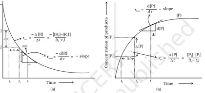
• Average rate over time interval Δt: rate = Δ[quantity]/Δt. For disappearance of A: average rate = −Δ[A]/Δt.
• Instantaneous rate at time t: rate = d[quantity]/dt (slope of tangent to concentration vs time curve).

Rate in terms of stoichiometry

For a reaction aA + bB → cC + dD, the rate is defined so that it is the same for all species:

rate = −(1/a)·d[A]/dt = −(1/b)·d[B]/dt = +(1/c)·d[C]/dt = +(1/d)·d[D]/dt.

Rate law (differential rate equation)

Experimentally determined expression relating rate to concentrations: rate = k [A]^m[B]ⁿ… where k is the rate constant and m, n are reaction orders (not necessarily equal to stoichiometric coefficients).

Reaction order and molecularity

• Order: sum of exponents (m + n + …) determined experimentally (can be 0, 1, 2, fractional).
• Molecularity: theoretical number of species colliding in an elementary step (always integer, e.g., unimolecular, bimolecular).

Integrated rate laws (for a single reactant A reacting alone)

• Zero-order: [A] = [A]₀ − kt. Half-life t_1/2 = [A]₀/(2k).
• First-order: ln[A] = ln[A]₀ − kt (or [A] = [A]₀ e^−kt). Half-life t_1/2 = ln 2 / k (independent of [A]₀).
• Second-order (2A → products or rate = k[A]²): 1/[A] = 1/[A]₀ + kt. Half-life t_1/2 = 1/(k [A]₀).

Rate constant and temperature dependence (Arrhenius equation)

k = A e^−E_a/(RT), where E_a is activation energy, A is frequency factor, R is gas constant, T is temperature (K). Plot ln k vs 1/T gives a straight line with slope −E_a/R.

Factors affecting rate

• Concentration (more reactants → higher frequency of collisions)
• Temperature (higher T → higher k and more molecules above E_a)
• Catalysts (lower E_a, provide alternate pathway)
• Pressure (affects rates for gases by changing concentrations)
• Surface area (for heterogeneous reactions; more area → faster rate)
• Solvent and presence of inhibitors/promoters

Methods of determining rate law

• Initial rates method: measure initial rate for different initial concentrations to find orders.
• Differential method: use instantaneous rates and log plots.
• Integrated method: fit concentration vs time data to integrated rate laws.

Qualitative theories

Collision theory: molecules must collide with sufficient energy and proper orientation to react. Transition-state theory: reaction proceeds through a high-energy activated complex.

Units

Units of rate: mol L⁻¹ s⁻¹ (or mol dm⁻³ s⁻¹). Units of k depend on overall order: e.g., first-order k: s⁻¹; second-order k: L mol⁻¹ s⁻¹; zero-order k: mol L⁻¹ s⁻¹.

Practical note: Rate laws must be determined experimentally. Stoichiometric equations do not by themselves give the rate law except for elementary steps.

Fig 3 — Educational Diagram: Factors Affecting Reaction Rate

Overview: The rate of a chemical reaction is the change in concentration of a reactant or product per unit time. Reaction rate depends on how often and how effectively reactant particles collide with sufficient energy and proper orientation (collision theory) and on the microscopic pathway (activation energy).

Main factors that affect reaction rate:

• Concentration (or concentration/partial pressure for gases): Higher concentration of reactants increases the frequency of effective collisions, usually increasing the rate. For a rate law Rate = k [A]^n [B]^m, increasing [A] changes the rate according to the order n.
• Temperature: Raising temperature increases kinetic energy of molecules, so more molecules exceed the activation energy (Ea). The quantitative relation is given by the Arrhenius equation k = A e^-Ea/RT. As T increases, k (and thus the rate) usually increases; a rough rule of thumb is that rate ~ doubles for each 10 °C rise (approximate).
• Presence of a catalyst: Catalysts provide an alternative pathway with lower activation energy, increasing the rate without being consumed. Enzymes are biological catalysts; heterogeneous catalysts provide surfaces for reactions (e.g., metal surfaces).
• Surface area (for heterogeneous reactions): For reactions involving a solid, greater surface area (e.g., powdered vs. chunk) exposes more reactive sites and increases rate.
• Pressure (for gases): Increasing pressure effectively increases gas concentrations, raising collision frequency and rate (important in gas-phase reactions).
• Nature (chemical identity) of reactants: Ionic reactions in solution (fast) vs. covalent bond-breaking steps (often slow). Strong bonds or complex reorganization slow rates.
• Solvent and medium effects: Solvent polarity, hydrogen bonding, and ionic strength can stabilize or destabilize transition states and reactants, changing rate. For example, SN1 reactions favor polar protic solvents.
• Light (photochemical reactions): Photons can promote molecules to excited states, enabling or accelerating reactions (e.g., photosynthesis, photodegradation).

Concepts to connect these factors:

• Collision theory: Rate ∝ collision frequency × fraction of collisions with energy ≥ Ea × orientation factor.
• Activation energy (Ea): Energy barrier that reactants must overcome for product formation. Lower Ea → higher rate.
• Arrhenius equation: k = A e^-Ea/RT relates temperature to the rate constant k. Taking ln gives ln k = ln A − Ea/RT, so a plot of ln k vs 1/T is a straight line with slope −Ea/R.
• Rate laws: Experimentally determined laws (Rate = k [A]^n [B]^m ...) show how concentration affects rate; reaction order (n, m) is not necessarily equal to stoichiometric coefficients.

Practical notes: To increase rate in industrial or lab processes you can raise concentration/pressure, increase temperature, use catalysts, increase surface area, or change solvent. Safety and selectivity must be considered when changing conditions.

Fig 4 — Educational Diagram: Rate Law and Rate Constant

What is rate law?
The rate law (or rate equation) expresses how the reaction rate depends on the concentrations of reactants (and sometimes products or catalysts) under given conditions. For a general reaction aA + bB -> products the rate law is written as:

rate = k [A]^m [B]ⁿ

Here k is the rate constant and m and n are the reaction orders with respect to A and B respectively. The overall order is (m + n). Orders are determined experimentally and need not equal stoichiometric coefficients except for elementary reactions.

Rate constant (k)
k is a proportionality constant that converts the concentration-dependent term into an actual rate. It depends on temperature, activation energy and the presence of catalysts but not on reactant concentrations. Increasing temperature generally increases k.

Determination of the rate law

• Initial rates method: measure initial rate for different initial concentrations, then compare how rate changes. If rate doubles when [A] doubles (others constant) then order in A is 1, etc. Using log form: log(rate) = log k + m log[A] + n log[B]. A plot of log(rate) vs log[A] gives slope = m.
• Integrated rate laws (monitor concentration vs time):
  • Zero order: [A] = [A]₀ - kt (straight line when [A] vs t)
  • First order: ln[A] = ln[A]₀ - kt (straight line when ln[A] vs t)
  • Second order: 1/[A] = 1/[A]₀ + kt (straight line when 1/[A] vs t)
• Half-life method: dependence of half-life on initial concentration distinguishes orders (t_1/2 independent of [A]₀ for first order, proportional to [A]₀ for zero order, inversely proportional to [A]₀ for second order).

Molecularity vs Order
Molecularity is the number of species that collide in an elementary step (unimolecular, bimolecular, termolecular) and is always a positive integer. Order is experimental and may be fractional, zero or an integer; it is the exponent in the rate law and applies to the overall reaction as observed.

Temperature dependence: Arrhenius equation
The temperature dependence of k is given by the Arrhenius equation:

k = A e^-E_a/(RT)

where A is the frequency (pre-exponential) factor, E_a is activation energy, R is gas constant and T is absolute temperature. A plot of ln k vs 1/T is linear with slope -E_a/R.

Pseudo-first-order reactions
When one reactant is present in large excess, its concentration changes little and can be treated as constant. The rate law simplifies to a pseudo-first-order form, e.g. rate = k' [A] where k' = k[B]_excess.

Relation to mechanism
The observed rate law constrains possible mechanisms. An elementary step has a rate proportional to the product of concentrations of species that collide in that step. Complex mechanisms are sequences of elementary steps; the slowest (rate-determining) step often controls the observed rate law.

Factors affecting rate constant and rate

• Concentration of reactants (affects rate, not k)
• Temperature (affects k via Arrhenius)
• Catalysts (increase k by lowering E_a)
• Physical state, surface area, pressure (for gases)

Useful practical notes for students

• Always determine orders experimentally; do not assume they equal stoichiometric coefficients unless the reaction is known to be elementary.
• Use linear plots for integrated laws to identify order: [A] vs t (zero), ln[A] vs t (first), 1/[A] vs t (second).
• Check units of k: they change with order. The general unit form is concentration^1-order time^-1.

Fig 5 — Educational Diagram: Order of a Reaction

Definition: The order of a reaction is the power to which the concentration of a reactant is raised in the rate law. The overall order is the sum of the powers (exponents) of all concentration terms in the experimentally determined rate equation. For a rate law rate = k[A]^m[B]^n, the overall order = m + n.

Key points:

• Order is determined experimentally (not from stoichiometry except for elementary reactions).
• Molecularity is a different concept: it applies to a single elementary step and is always an integer (unimolecular, bimolecular...). Order can be fractional or negative.
• Pseudo-order: when one reactant is in large excess, its concentration is effectively constant and the reaction can be treated as a lower-order (pseudo) reaction.

How to determine order experimentally:

• Method of initial rates: measure initial rate for different initial concentrations. If rate ∝ [A]^x, then log(rate) vs log([A]) slope = x.
• Integrated rate laws: fit concentration vs time data to the integrated forms (zero, first and second order) and see which gives a straight line.

Integrated rate laws (for a single reactant A):

• Zero order: [A] = [A]₀ − kt (linear plot: [A] vs t)
• First order: ln[A] = ln[A]₀ − kt (linear plot: ln[A] vs t)
• Second order (2A → products): 1/[A] = 1/[A]₀ + kt (linear plot: 1/[A] vs t)

Half-life (t_1/2) dependences:

• Zero order: t_1/2 = [A]₀ / (2k) (depends on initial concentration)
• First order: t_1/2 = ln2 / k (independent of [A]₀)
• Second order: t_1/2 = 1 / (k [A]₀) (depends on [A]₀)

Units of rate constant (k): dependent on overall order n. General rule: units = concentration^(1−n) time^(−1). Examples: zero-order: mol L⁻¹ s⁻¹; first-order: s⁻¹; second-order: L mol⁻¹ s⁻¹.

Remarks: Orders can be integers, fractions or negative values depending on mechanism. For multi-step mechanisms, the observed rate law reflects the rate-determining step(s). Always determine order from experiments.

Fig 6 — Educational Diagram: Molecularity of a Reaction

Definition: Molecularity of an elementary reaction is the number of reactant particles (molecules, atoms or ions) that must collide simultaneously to produce the reaction. It applies only to an elementary step and is always a positive integer (1, 2, 3,...).

Types:

• Unimolecular (molecularity = 1): A single species undergoes transformation by itself (e.g., isomerisation or decomposition of a single molecule).
• Bimolecular (molecularity = 2): Two species collide and react (common case).
• Termolecular (molecularity = 3): Three species must collide simultaneously – rare because simultaneous three-body collisions are unlikely; often observed as a three-body recombination where a third body stabilises the product.

Relation to rate law (elementary step): For an elementary reaction, the rate law follows directly from molecularity because each colliding particle contributes one concentration factor. For example, for the elementary step aA + bB → products (where a and b are small integers representing simultaneous colliding species), molecularity = a + b and rate = k[A]^a[B]^b.

Important notes:

• Molecularity is defined only for elementary steps, not for overall (multi-step) reactions.
• Molecularity is always an integer; it cannot be zero or fractional. Reaction order, by contrast, is determined experimentally for the overall rate law and may be fractional or zero.
• Termolecular elementary steps are rare; many apparent three-body overall reactions proceed by two-step mechanisms involving an intermediate and a stabilising third body.

Comparison with order of reaction (brief): Molecularity (theoretical, integer, elementary step) vs Order (experimental, sum of exponents in the rate law, may be non-integer). Only for true elementary steps does the order equal molecularity.

Fig 7 — Educational Diagram: Differential and Integrated Rate Laws

Overview
Differential and integrated rate laws describe how the rate of a chemical reaction depends on reactant concentrations and how concentrations change with time.

Differential rate law (rate equation)
For a general reaction aA + bB → products the instantaneous rate r is given by the differential rate law:

r = k [A]^m [B]^n

Here k is the rate constant and m, n are the orders of the reaction with respect to A and B (determined experimentally, not necessarily equal to stoichiometric coefficients). If the reaction involves only A, the differential law becomes:

r = - (1/a) d[A]/dt = k [A]^m

Finding orders
Use the method of initial rates or log plots: taking logs gives log r = log k + m log[A] + n log[B], so slopes of log–log plots give orders.

Integrated rate laws (single-reactant cases)
Integrated laws are obtained by separating variables and integrating the differential law; they relate concentration to time.

Zero order (m = 0)
Differential: r = -d[A]/dt = k
Integrated: [A] = [A]₀ − k t
Half-life: t_1/2 = [A]₀/(2k) (depends on initial concentration)

First order (m = 1)
Differential: r = -d[A]/dt = k [A]
Integrated: ln[A] = ln[A]₀ − k t (or [A] = [A]₀ e^−kt)
Half-life: t_1/2 = ln 2 / k (independent of [A]₀)

Second order (m = 2, for 2A → products)
Differential: r = -d[A]/dt = k [A]²
Integrated: 1/[A] = 1/[A]₀ + k t
Half-life: t_1/2 = 1 / (k [A]₀)

Notes
- Units of k depend on overall order: zero-order (mol L⁻¹ s⁻¹), first-order (s⁻¹), second-order (L mol⁻¹ s⁻¹).
- Reaction order is empirical; molecularity is theoretical (elementary steps only).
- Pseudo-first-order kinetics: if one reactant is in large excess its concentration is effectively constant and a higher-order reaction can behave as first-order in the limiting reactant.

How to determine order experimentally
1) Initial rates: vary concentrations, measure initial rate, use log–log plot to get slopes (orders).
2) Integrated methods: try plotting concentration vs t (zero-order), ln[A] vs t (first-order), or 1/[A] vs t (second-order); the plot that gives a straight line indicates the order.

Practical use
Integrated laws let you predict concentration at time t, compute half-lives, and compare experimental data to decide kinetics and mechanisms.

Fig 8 — Educational Diagram: Half-life (t1/2) Expressions

Definition: The half-life (t1/2) of a reactant A is the time required for its concentration to decrease to half of its initial value: [A](t1/2) = [A]0/2.

Context and importance: Half-life helps characterize the speed of a reaction and compare kinetics. For some reaction orders (notably first order) t1/2 is independent of the initial concentration, which has practical consequences (e.g., radioactive decay, drug elimination).

Rate law and integrated forms (brief): For a homogeneous reaction where rate = −d[A]/dt = k[A]^n, integrated rate expressions allow solving for [A] as a function of time and hence for t1/2.

Derivations for common orders:

• Zero order (n = 0): Integrated form: [A] = [A]0 − kt. Set [A] = [A]0/2 at t = t1/2: kt1/2 = [A]0/2 ⇒ t1/2 = [A]0/(2k). (t1/2 depends on [A]0.)
• First order (n = 1): Integrated form: ln[A] = ln[A]0 − kt. Set [A] = [A]0/2: ln(1/2) = −kt1/2 ⇒ t1/2 = ln2 / k (≈ 0.693/k). (Independent of [A]0.)
• Second order (n = 2, for 2A → products or rate ∝ [A]^2): Integrated form: 1/[A] = kt + 1/[A]0. At t1/2, 1/([A]0/2) = kt1/2 + 1/[A]0 ⇒ t1/2 = 1/(k[A]0). (Depends on [A]0.)
• General n (n ≠ 1): Integrated form gives ([A]^(1−n) − [A]0^(1−n)) = (n−1)k t. Put [A] = [A]0/2 and solve to get
  t1/2 = (2^(n−1) − 1) / ((n−1) k [A]0^(n−1)). This formula reduces to the above cases for n = 0 and n = 2.

Pseudo-first-order reactions: If one reactant is in large excess so its concentration is effectively constant, the reaction behaves like first order with an effective rate constant k' = k[excess]^(m). Then t1/2 = ln2 / k'.

Key points to remember: (1) First-order t1/2 is constant and independent of [A]0; (2) For zero and second order, t1/2 depends on [A]0 (linearly for zero order, inversely for second order); (3) t1/2 formulas come directly from the integrated rate laws.

Fig 9 — Educational Diagram: Methods to Determine Order and Rate Constant

Overview: Chemical kinetics determines how fast a reaction proceeds (rate) and how the rate depends on reactant concentrations (order). Experimental methods find the rate law: rate = k [A]^m [B]^n ...; the exponents (m, n, ...) give the order and k is the rate constant.

Main experimental methods

• Method of initial rates (rate method)

  Measure the initial rate (when product formation is negligible) for several experiments with different starting concentrations. Keeping other reactants fixed while varying one allows determination of that reactant's order by comparing rates. If rate ∝ [A]^m, then for two experiments: rate1/rate2 = ([A]1/[A]2)^m. Taking logs: m = log(rate1/rate2) / log([A]1/[A]2). Repeat for each reactant.

• Differential method

  Compute instantaneous rates (d[P]/dt or -d[A]/dt) from concentration vs time data and plot log(rate) vs log(concentration). The slope gives the order (log(rate) = m log[A] + constant). Requires precise derivative estimates and noise reduction.

• Integrated rate law (graphical) method

  Use integrated forms for simple orders and test linearity of transformed data: for a single reactant A:

  • Zero order: [A] = -kt + [A]0 → plot [A] vs t (straight line, slope = -k).
  • First order: ln[A] = -kt + ln[A]0 → plot ln[A] vs t (straight line, slope = -k).
  • Second order (2A → products or rate = k[A]^2): 1/[A] = kt + 1/[A]0 → plot 1/[A] vs t (straight line, slope = k).

  For reactions with multiple reactants, hold others in large excess (isolation/pseudo-first-order) so their concentrations ≈ constant and treat the reaction effectively as single-reactant to apply integrated forms.

• Method of isolation / pseudo-first-order method

  Make one (or more) reactant(s) present in large excess so their concentration is effectively constant. The rate law simplifies (e.g., rate = k'[A]^m with k' = k[B]^n), and usual integrated/graphical tests yield m and k'. Knowing excess concentrations allows recovery of true k.

• Half-life method

  Measure the time required for concentration to fall to half the initial value (t_1/2). Dependence of t_1/2 on [A]0 identifies order:

  • First order: t_1/2 = ln 2 / k (independent of [A]0).
  • Second order (single reactant): t_1/2 = 1 / (k [A]0) (depends on [A]0).
  • Zero order: t_1/2 = [A]0 / (2k).
• Non-linear regression / modern fitting

  Fit concentration-vs-time data directly to proposed rate-law solutions (numerically or using least-squares) to obtain order(s) and best-fit k. This is robust when noise exists or reactions are complex.

Determining k from plots: When the correct integrated plot is linear, the slope gives k (or -k). Example: slope of ln[A] vs t = -k (first-order), slope of 1/[A] vs t = +k (second-order), slope of [A] vs t = -k (zero-order).

Temperature dependence: Once k is known at several temperatures, use the Arrhenius equation: k = A e^-Ea/RT. A plot of ln k vs 1/T gives slope = -Ea/R and intercept = ln A.

Practical notes:

• Initial rates avoid complications from reverse reactions and product effects.
• Pseudo-first-order is widely used (e.g., hydrolysis in water where water is in great excess).
• Graphical integrated tests are simple and visual; modern practice favors numerical fitting for precision.

Fig 10 — Educational Diagram: Pseudo First-Order Reactions

Definition: A pseudo first-order reaction is a reaction that is actually of higher order (commonly second order) but under experimental conditions behaves like a first‑order reaction because the concentration of one (or more) reactants is kept in large excess and therefore remains effectively constant during the reaction.

Concept and derivation (typical bimolecular case):

Consider a bimolecular reaction: A + B → products with rate law rate = k[A][B]. If [B]0 >> [A]0, then [B] changes negligibly during the reaction and can be approximated by its initial value [B]0. Substituting this constant into the rate law gives:

rate = k[A][B] ≈ k[A][B]0 = k'[A]

where k' = k[B]0 is the pseudo-first-order rate constant. This converts the kinetics to a first-order form in [A].

Integrated form (same as first-order):

ln[A]t = ln[A]0 − k' t

or [A]t = [A]0 e^(−k' t)

Half-life (for the pseudo-first-order decay of A):

t1/2 = ln 2 / k'

How to get the true rate constant k experimentally:

1. Carry out several experiments with different large excess concentrations of B ([B]0 values).
2. For each experiment obtain k' from the slope of ln[A] vs t (slope = −k').
3. Plot k' versus [B]0. The plot should be linear: k' = k[B]0. The slope of this line gives the true bimolecular rate constant k.

When else is this used? It applies whenever one reactant (or catalyst) concentration is held effectively constant: e.g., solvent (water) in large excess, catalysts present at low constant concentration, or any situation where one species changes negligibly over the time scale of observation. Pseudo‑order kinetics simplifies analysis and is widely used in lab kinetics.

Limitations and assumptions:

• [B] must remain essentially constant over the measured time interval.
• Temperature and ionic strength (if relevant) must be constant.
• If [B] is not large enough, the approximation fails and full higher‑order analysis is needed.

Fig 11 — Educational Diagram: Reaction Mechanisms and Elementary Steps

What is a reaction mechanism?
A reaction mechanism is a sequence of one or more elementary steps that shows the actual path by which reactants are converted into products. Each elementary step is a single molecular event (bond breaking/forming) and has its own rate law.

Elementary step and molecularity
An elementary step is elemental in that its stoichiometry equals the molecularity of that step:

• Unimolecular: A → products (molecularity = 1)
• Bimolecular: A + B → products (molecularity = 2)
• Termolecular: A + B + C → products (molecularity = 3) — rare

For an elementary step the rate law can be written from the molecularity: rate = k[A]^m[B]^n (where m, n are the stoichiometric coefficients of species participating in that elementary step).

Reaction order vs molecularity
Molecularity is a theoretical property of an elementary step and is always an integer. Reaction order is determined experimentally for the overall reaction and can be non-integer. For a single-step (elementary) reaction, order = molecularity; for multi-step (complex) reactions the overall order may differ.

Complex reactions — rate-determining step (RDS)
Most reactions proceed by several elementary steps. The slowest step among these is the rate-determining step (RDS) and usually controls the observed rate law. If the RDS is elementary, the rate law usually follows the stoichiometry of that step. However, intermediates produced/consumed in other steps may require approximations (steady-state or pre-equilibrium) to derive the observed rate law.

Intermediates, transition states and catalysts
Intermediates are species produced in one step and consumed in another — they do not appear in the overall equation. Transition states are high-energy states along a step and are not isolable. A catalyst participates in elementary steps but is regenerated overall and does not appear in the net equation.

Steady-state approximation (SSA)
For a short-lived intermediate I, SSA assumes its concentration remains approximately constant: d[I]/dt ≈ 0. This lets you solve for [I] and substitute into the RDS expression to obtain the observable rate law.

Pre-equilibrium approximation
If an early step is fast and reaches equilibrium before the RDS, you can use its equilibrium constant (K = k_fast/k_-fast) to express intermediate concentrations in terms of reactants, then insert into the RDS rate expression.

How to determine a plausible mechanism

1. Use experimental rate law as constraint.
2. Propose elementary steps whose combined stoichiometry gives the overall reaction.
3. Identify intermediates and apply RDS / SSA / pre-equilibrium to derive the rate law; compare with experiment.
4. Refine mechanism as needed (catalysts, chain steps, surface adsorption).

Important conceptual points

• Rate laws for elementary steps follow molecularity; overall rate laws may not.
• RDS often corresponds to the largest activation energy (highest energy transition state) on the energy profile.
• Chain reactions (free radical mechanisms) have initiation, propagation and termination steps and often show complex kinetics.

Fig 12 — Educational Diagram: Steady State Approximation and Pre-equilibrium Approaches

Overview
Both methods are approximations used in chemical kinetics to obtain simple rate laws for mechanisms involving short‑lived intermediates. They let us eliminate intermediate concentrations to express the rate in terms of reactants (observable species).

Steady State Approximation (SSA)
Definition: For an intermediate I produced and consumed in a mechanism, the steady state assumption sets its net rate of change to zero: d[I]/dt ≈ 0. This is valid when I is formed and consumed rapidly so that its concentration remains small and approximately constant during the reaction.

Procedure (typical):
1) Write differential rate expressions for all species using elementary steps.
2) For the intermediate(s) set d[I]/dt = 0 and solve for [I] in terms of reactants.
3) Substitute [I] into the expression for the rate of product formation to obtain the observable rate law.

Illustrative mechanism (consecutive first order):
A --(k1)--> I --(k2)--> P
Rate expressions: d[I]/dt = k1[A] - k2[I]. SSA: 0 = k1[A] - k2[I] so [I] = (k1/k2)[A]. Rate of P formation: r = k2[I] = k1[A]. In this limit the overall rate is first order with respect to A (when the second step is much faster so I does not accumulate).

When to use SSA
Use SSA when intermediates are short‑lived and their concentrations remain small compared with reactants. SSA is widely used for radical chain mechanisms and enzyme catalysis.

Pre-equilibrium Approach
Definition: If an early step (or set of steps) is fast and reversible and establishes an equilibrium between reactants and an intermediate B, and a subsequent step is slow (rate‑determining), we can assume the fast step is at equilibrium (pre‑equilibrium). Then use equilibrium relations to eliminate [B].

Typical mechanism: A <--(k-1)--> B --(k2)--> P with k2 ≪ k-1.
Pre‑equilibrium: K = [B]/[A] = k1/k-1 so [B] = K[A]. Rate of product formation: r = k2[B] = k2 K [A]. The overall rate is first order in A with an apparent rate constant kapp = k2 K.

When to use pre‑equilibrium
Use it when the forward and reverse of the first step are fast compared with the slow step that follows, so the intermediate and reactant rapidly establish an equilibrium.

Common classroom examples
- Enzyme catalysis (Michaelis–Menten): E + S <--> ES --(k2)--> E + P. Often treated by SSA for [ES], producing the Michaelis–Menten equation.
- SN1 organic substitution: R–LG <--> R+ + LG- (fast equilibrium or rate‑determining ionization depending on case) then R+ + Nu -> product (pre‑equilibrium used when ionization is fast reversible).
- Atmospheric chemistry (Chapman mechanism for ozone): atomic O is an intermediate treated by SSA.

Limitations
Both approximations are not universally valid. Check conditions (relative magnitudes of rate constants and timescales) before applying. If intermediates accumulate or the ‘‘fast’’ step is not sufficiently fast, results will be inaccurate.

Fig 13 — Educational Diagram: Chain Reactions

Definition: A chain reaction is a reaction in which reactive intermediates (chain carriers, usually free radicals, ions or atoms) produced in one step initiate further reaction steps, so that a sequence (chain) of propagation steps occurs before the chain is terminated.

Stages of a chain reaction:

• Initiation: formation of reactive chain carriers. Example: Br2 --(hν)--> 2 Br·
• Propagation: chain carriers react with stable molecules to form products and regenerate carriers. Example (H2 + Br2): Br· + H2 -> HBr + H· ; H· + Br2 -> HBr + Br·
• Termination: two chain carriers combine or are removed, stopping the chain. Example: Br· + Br· -> Br2 ; H· + Br· -> HBr

Characteristics:

• Few initiation events can produce many product molecules (large chain length).
• Reaction rate may show unusual orders (fractional or near zero order) because radical concentrations are governed by steady-state balance between formation and removal.
• Chain-branching (where carriers produce more than one new carrier) can cause explosive increases in rate (combustion, detonations).

Steady-state concept for chain carriers (qualitative): Because chain carriers are highly reactive, their concentrations are typically small and approximately constant during most of the reaction. Using the steady-state approximation (rate of formation ≈ rate of removal) for radicals allows derivation of observable rate laws that often show fractional orders with respect to some reactants.

Illustrative derivation (sketch) — H2 + Br2 reaction: Initiation (photochemical): Br2 --(hν)--> 2 Br· (rate of initiation = q[Br2]). Propagation: Br· + H2 -> HBr + H· (k1); H· + Br2 -> HBr + Br· (k2). Termination: Br· + Br· -> Br2 (k3[Br·]^2). Applying steady-state for Br· (formation ≈ removal) gives [Br·] proportional to sqrt(q[Br2]/k3). Product formation rate ~ k1[Br·][H2] so experimentally rate ∝ [H2][Br2]^(1/2). This explains the observed fractional order in Br2.

Chain length: Chain length (ν) = (number of molecules of product formed by propagation)/(number of initiation events) = rate of product formation / rate of initiation. Large ν means efficient propagation relative to initiation/termination.

Chain branching: If a propagation step produces more than one active carrier (e.g., A· -> 2 A·), the carrier population can grow exponentially leading to very rapid or explosive reaction rates (important in combustion: H + O2 branching sequences).

Importance: Chain mechanisms explain many free-radical reactions (halogenation of alkanes, free-radical polymerization), combustion chemistry, atmospheric radical chemistry (ozone depletion), and nuclear fission (neutron-induced chain reactions).

Fig 14 — Educational Diagram: Collision Theory of Rate of Reaction

Basic idea: Collision theory explains how and why chemical reactions occur by considering collisions between reactant particles (molecules/atoms/ions). For a reaction to occur, reactant particles must (i) collide, (ii) collide with sufficient energy (equal to or greater than the activation energy, E_a), and (iii) have a correct relative orientation during the collision.

Key postulates:

• Reactant particles move randomly and collide with one another; only collisions can lead to reactions.
• Not all collisions lead to products. Only a fraction are effective collisions — those with energy ≥ E_a and correct orientation.
• The number of collisions per unit time depends on concentration (or pressure), temperature, and particle size.

Collision frequency and effective collisions: The total collision frequency (Z) gives the number of collisions per unit volume per unit time. The fraction of collisions having energy ≥ E_a is given approximately by the Boltzmann factor, exp(−E_a/RT). A steric (orientation) factor p (0 < p ≤ 1) accounts for the fraction of collisions with correct orientation. Thus the number of effective collisions per unit volume per unit time is approximately p Z exp(−E_a/RT).

Relation to rate constant: The rate constant k is proportional to the number of effective collisions per reacting pair. This leads to the Arrhenius form k = A e^−E_a/RT, where A (the pre-exponential factor) ≈ p Z (for bimolecular gas-phase reactions it depends on collision frequency and orientation). The Arrhenius equation quantifies the strong temperature dependence of k.

Temperature effect: Raising temperature increases both collision frequency (slightly) and, much more importantly, the fraction of molecules with energy ≥ E_a (exponentially larger), so reaction rates rise rapidly with temperature. This is visualized by the Maxwell–Boltzmann energy distribution shifting and broadening with temperature, increasing the area of the curve beyond E_a.

Effects of concentration/pressure, catalysts, and surface area:

• Increasing concentration (or gas pressure) raises particle number density, increasing collision frequency and rate.
• Catalysts lower the activation energy (or provide an alternate pathway), increasing the fraction of effective collisions (larger k) without being consumed.
• In heterogeneous reactions, increasing surface area increases the number of reactive collisions at the interface.

Limitations: Collision theory works best for simple gas-phase bimolecular reactions. It is less accurate for complex reactions, solution-phase reactions where solvent effects and diffusion control dominate, and enzyme-catalyzed reactions that involve specific binding steps.

Summary (conceptual): Reaction rate ∝ (collision frequency) × (fraction with E ≥ E_a) × (orientation probability). Quantitatively this leads to k ≈ p Z e^−E_a/RT and to the experimentally useful Arrhenius equation k = A e^−E_a/RT.

Fig 15 — Educational Diagram: Activation Energy and Activated Complex

Activation Energy (E_a): Activation energy is the minimum energy that reacting molecules must possess for a successful collision that leads to product formation. It is an energy barrier separating reactants and products on the potential energy surface. Only collisions in which the colliding molecules have energy equal to or greater than E_a can produce products.

Activated Complex (Transition State): The activated complex (or transition state) is a short‑lived, high‑energy arrangement of atoms that exists at the top of the activation barrier during a chemical reaction. It is not an isolable intermediate; it has partial bonds that are in the process of breaking and forming. The activated complex corresponds to the maximum on a potential energy vs reaction‑coordinate diagram.

Connection with Reaction Rate and Temperature: According to collision theory and the Arrhenius equation, the rate constant k depends on the fraction of molecules having energy ≥ E_a. The Boltzmann factor e^−E_a/RT gives the fraction of molecules with sufficient energy at temperature T. Increasing temperature increases this fraction, thus increasing the rate.

Effect of Catalysts: A catalyst provides an alternative pathway with a lower activation energy (lower energy peak). It stabilizes one or more transition states or provides a different transition state, increasing the rate without changing the overall enthalpy change (ΔH) of the reaction.

Important conceptual points:

• E_a is always positive for elementary reactions that require an energy barrier; some barrierless or barrier‑free reactions have negligible E_a.
• The activated complex is a transient state at the energy maximum and differs from a reaction intermediate (which can sometimes be isolated and corresponds to a local energy minimum).
• Forward and reverse activation energies differ: E_a,f for reactants → products and E_a,r for products → reactants; their difference equals the enthalpy change ΔH (E_a,f − E_a,r = ΔH).

Fig 16 — Educational Diagram: Arrhenius Equation

Definition
The Arrhenius equation gives the temperature dependence of the rate constant (k) of a chemical reaction. It relates k to an activation energy (E_a) and a frequency (pre-exponential) factor (A):

k = A · e^−E_a/(RT)

Here R is the gas constant and T the absolute temperature (K). The equation arises from the idea that only a fraction of collisions have energy equal to or greater than the activation energy; that fraction is proportional to e^−E_a/(RT). A represents the frequency of effective collisions (orientation and collision frequency).

Linear (log) form and use
Taking natural logs gives a linear relationship useful in analysis:

ln k = ln A − E_a/(RT)

Plotting ln k (y-axis) versus 1/T (x-axis) yields a straight line with slope = −E_a/R and intercept = ln A. This is called the Arrhenius plot and is used to determine E_a and A experimentally.

Two-point form (useful for calculations)
From the Arrhenius equation for two temperatures T₁ and T₂:

ln(k₂/k₁) = −(E_a/R) · (1/T₂ − 1/T₁)

This is often used to compute E_a or to estimate how k changes with T.

Physical meaning & points to remember

• E_a (activation energy) is the minimum energy barrier that reactant molecules must overcome to form products. Units: J mol⁻¹ (or kJ mol⁻¹).
• A (frequency factor) reflects collision frequency and proper orientation; units same as k (depend on reaction order).
• When using R = 8.314 J mol⁻¹ K⁻¹, ensure E_a is in J mol⁻¹ not kJ mol⁻¹.
• A catalyst lowers E_a, producing a less steep slope on an Arrhenius plot and increasing the rate constant at a given T.
• Rule of thumb: for many reactions a 10 °C (≈10 K) increase roughly doubles or triples the rate — this is qualitative and depends on E_a.

Relation to molecular ideas
From kinetic theory / Maxwell–Boltzmann distribution: the fraction of molecules with energy ≥ E_a is proportional to e^−E_a/(RT). Multiplying this fraction by an attempt frequency (A) gives the rate constant form.

Fig 17 — Educational Diagram: Temperature Dependence of Rate Constant

Overview

The rate constant k of a chemical reaction strongly depends on temperature. Two main theoretical explanations are used: the Arrhenius empirical relationship (based on collision theory ideas) and the Transition State (Eyring) theory. Increasing temperature increases the fraction of molecules that have enough energy to overcome the activation energy barrier, so k usually increases with T.

Arrhenius equation (physical meaning)

Arrhenius proposed that the rate constant k varies with temperature according to
k = A e^{-E_a/(RT)} where A is the pre-exponential (frequency) factor, E_a is the activation energy (J mol^-1), R is the gas constant (8.314 J mol^-1 K^-1) and T is absolute temperature (K). Physically, A accounts for collision frequency and correct orientation of colliding molecules; e^{-E_a/(RT)} is the fraction of collisions with energy ≥ E_a.

Linear (log) form — useful for experimental determination

Taking natural logs gives a straight-line equation:
ln k = ln A - E_a/(RT) A plot of ln k versus 1/T (Arrhenius plot) is a straight line with slope −E_a/R and intercept ln A. From the slope you can calculate E_a.

Two-point Arrhenius relation

If k₁ at T₁ and k₂ at T₂ are known,
ln(k_2/k_1) = -E_a/R (1/T_2 - 1/T_1) This form is commonly used to find E_a from two rate constants or to predict k at a new temperature.

Temperature coefficient (Q10) and rule-of-thumb

The temperature coefficient Q₁₀ = k(T+10°C)/k(T) quantifies how rate changes with a 10 °C rise. Many ordinary chemical reactions have Q₁₀ ≈ 2 (rate roughly doubles per 10 °C) — this follows from the Arrhenius equation for typical activation energies (≈40–80 kJ mol^-1) at room temperature. Q₁₀ can be computed from Arrhenius as
Q_10 = exp[ E_a/R (1/T - 1/(T+10) ) ]

Transition state (Eyring) theory — microscopic form

Transition state theory gives a slightly different, more microscopic expression:
k = (k_B T/h) e^{-ΔG^‡/(RT)} = (k_B T/h) e^{ΔS^‡/R} e^{-ΔH^‡/(RT)} where k_B is Boltzmann constant, h is Planck constant, ΔG^‡ is the Gibbs free energy of activation, ΔH^‡ is the enthalpy of activation and ΔS^‡ is the entropy of activation. This form separates the enthalpic barrier (ΔH^‡) and entropic contributions (ΔS^‡) to the rate.

Relation between Arrhenius and Eyring parameters

Comparing the two forms gives an approximate relation E_a ≈ ΔH^‡ + RT (so E_a is close to the activation enthalpy plus RT). The pre-exponential factor A relates to (k_B T/h) e^{ΔS^‡/R}.

Practical consequences

• Small increases in T often produce large increases in k for reactions with sizable E_a (exponential dependence).
• Low activation energy reactions show weaker temperature dependence.
• Enzyme-catalyzed reactions: k increases with T up to an optimum; above that proteins denature and rate falls (non-Arrhenius behaviour).

Example numeric check of the 10 °C rule

For E_a = 50 kJ mol^-1, T = 298 K:
Q_10 = exp[50000/8.314 (1/298 - 1/308)] ≈ exp(0.654) ≈ 1.92 So roughly a doubling of rate per 10 °C increase.

Summary

Temperature affects k exponentially via the Arrhenius factor e^{-E_a/(RT)}. The Arrhenius plot (ln k vs 1/T) gives E_a and A. Transition state theory gives deeper insight by separating enthalpic and entropic contributions to the activation barrier.

Fig 18 — Educational Diagram: Catalysis

Definition : Catalysis is the increase (or decrease) in the rate of a chemical reaction brought about by the addition of a substance called a catalyst. A catalyst provides an alternative reaction pathway with a lower activation energy and is not consumed (net) in the overall reaction.

How catalyst works : A catalyst lowers the activation energy (E_a) required for the reaction by offering an alternate mechanism (often via adsorbed intermediates or an enzyme–substrate complex). Because of the lower E_a, a larger fraction of collisions leads to product formation and the rate constant k increases (Arrhenius behaviour). The overall enthalpy change (ΔH) remains unchanged.

Key features :

• Catalyst is not consumed in the overall reaction (it may be temporarily changed in intermediate steps).
• It changes the rate, but not the equilibrium position (it speeds up both forward and reverse reactions equally).
• It may change the reaction mechanism and therefore can change the observed rate law.

Types of catalysis :

• Homogeneous catalysis — catalyst and reactants are in the same phase (example: acid-catalysed esterification with H⁺).
• Heterogeneous catalysis — catalyst and reactants are in different phases (typically solid catalyst + gas/liquid reactants; example: hydrogenation on Ni or the Haber process on Fe).
• Enzyme catalysis (biocatalysis) — highly specific biological catalysts (enzymes) that follow kinetics often described by the Michaelis–Menten model.
• Autocatalysis — one of the products acts as a catalyst for the reaction (rate increases as product builds up).
• Positive (accelerating) and negative (inhibiting) catalysis — catalysts that increase or decrease rate respectively. Catalyst poisoning is an extreme form of inhibition.

Important practical points : Promoters and supports are used in industry to increase activity and stability. Poisoning (e.g., sulfur or CO on metal surfaces) reduces catalyst activity. Turnover number (TON) and turnover frequency (TOF) are measures of catalytic performance:

• TON = moles of product formed per mole of catalyst (over a period).
• TOF = moles of product formed per mole of catalyst per unit time.

Enzyme example & kinetics : Enzymes form an enzyme–substrate complex (ES). The Michaelis–Menten equation describes initial rate v versus substrate [S]: v = V_max[S]/(K_m + [S]). Enzymes are highly specific and operate under mild conditions.

Applications (brief) : Haber process (Fe catalyst) for NH₃ synthesis, catalytic converters (Pt/Pd/Rh) for automobile exhaust cleanup, hydrogenation of vegetable oils (Ni), decomposition of H₂O₂ by catalase (biological), and industrial oxidation/hydrogenation processes (heterogeneous catalysts).

Fig 19 — Educational Diagram: Enzyme Kinetics (Basic)

What is enzyme kinetics? Enzyme kinetics studies the rates of chemical reactions catalyzed by enzymes and how those rates depend on variables such as substrate concentration, enzyme concentration, temperature, pH and inhibitors.

Basic reaction scheme: E + S ↔ ES → E + P, where E = enzyme, S = substrate, ES = enzyme-substrate complex, P = product. Rate constants: k1 (formation of ES), k-1 (dissociation back to E + S) and k2 (conversion of ES to product).

Steady-state (Briggs–Haldane) assumption: After a short initial transient the concentration of ES remains approximately constant (d[ES]/dt ≈ 0). Using this one derives the Michaelis–Menten equation for the initial rate v0:

v = Vmax [S] / (Km + [S])

Here Vmax is the maximum rate achieved when the enzyme is saturated with substrate and Km (Michaelis constant) is defined as Km = (k-1 + k2)/k1. Km has units of concentration and is the substrate concentration at which v = Vmax/2; it is often interpreted as a measure of the enzyme's affinity for substrate (lower Km = higher apparent affinity under many conditions).

Other important relationships: Vmax = k2 [E]total (often written Vmax = kcat [E]total where kcat is the turnover number, the number of substrate molecules converted per enzyme molecule per unit time). Catalytic efficiency is kcat/Km and is useful for comparing enzymes or substrates when [S] is much less than Km.

Measuring kinetics: Initial-rate (v0) measurements are made at several [S] values, then fitted to the Michaelis–Menten equation. A common linear transformation is the Lineweaver–Burk (double-reciprocal) plot: 1/v = (Km/Vmax)(1/[S]) + 1/Vmax, which gives a straight line to estimate Km and Vmax (y-intercept = 1/Vmax, x-intercept = -1/Km).

Effect of inhibitors (basic): Competitive inhibitors increase apparent Km (need more substrate to reach half Vmax) but do not change Vmax. Noncompetitive inhibitors reduce Vmax but do not change Km. Mixed inhibition affects both. These changes are conveniently visualized on Michaelis–Menten and Lineweaver–Burk plots.

Assumptions & limits: Michaelis–Menten applies to initial-rate conditions, single-substrate reactions (or treated as effective single-substrate), and when steady-state approximation holds. Real enzymes may show cooperativity, multi-substrate kinetics, or allosteric regulation that deviate from simple MM behavior.

Fig 20 — Educational Diagram: Experimental Techniques for Kinetic Measurements

Overview: Chemical kinetics studies the speed of chemical reactions and the factors that affect it. Experimental techniques measure how concentration, pressure, mass, colour or conductivity change with time so that rate laws, orders and rate constants can be determined.

Common experimental techniques (what is measured and typical apparatus):

• Spectrophotometry (colorimetric): measures absorbance (A) vs time using a UV–Vis spectrophotometer. Suitable when reactant or product absorbs light. Uses Beer–Lambert law (A ∝ concentration).
• Conductometry: measures electrical conductance vs time when ionic composition changes (e.g., acid–base hydrolysis, ionic product formation).
• Manometric / Gas collection: measures pressure or volume of gas produced or consumed vs time using a manometer, gas syringe or burette (useful for gaseous reactions).
• Gravimetric / Mass change: measures mass loss/gain of reaction mixture (e.g., gas evolution or precipitation) on a balance.
• Titration (discrete sampling): withdraw samples at intervals, quench reaction, and titrate to find concentration vs time (common in labs for many liquid-phase reactions).
• Polarimetry: measures optical rotation vs time when chiral concentrations change.
• Stopped-flow and flash photolysis: for very fast reactions (ms or μs) by rapid mixing or light-triggered start and continuous detection (often spectroscopic).
• Clock reactions: determine time to a sudden observable event (e.g., colour change) as function of initial concentrations to deduce rate law.

Determining rate law and k experimentally:

• Initial rate method: keep all but one reactant constant, measure initial rate for varied concentrations. Use rate ∝ [A]^n to find order n (log-log plot of rate vs [A]).
• Integrated rate laws: follow concentration vs time and fit to integrated forms (zero/first/second order) to obtain k and order. Compare linearity of plots described below.
• Pseudo-first-order method: one reactant in large excess so its concentration is effectively constant; reduces multi-reactant rate law to first order in the limiting reactant, simplifying analysis (common for hydrolysis/oxidation studies).

Practical points & controls:

• Maintain constant temperature (use thermostated baths) because k is temperature dependent.
• Use quenching or rapid sampling to stop reaction at sampling times for titrations.
• Calibrate instruments (spectrophotometer, conductometer) and confirm Beer–Lambert law holds for concentration range used.
• Account for side reactions, mixing times (important for fast kinetics), and systematic errors (e.g., evaporation in gas-collection).

Link with theory: measured concentration/time data are analysed using rate expressions and integrated laws to extract reaction order(s), k and activation energy (from temperature dependence via Arrhenius plot).

Fig 21 — Educational Diagram: Units and Dimensions of Rate Constant

What is the rate constant (k)?
The rate constant k appears in the rate law: rate = k [A]^a [B]^b ... . It is a proportionality constant that depends on temperature and activation energy (Arrhenius behaviour) but not on reactant concentrations. Its numerical value and units change with the overall order (n = a + b + ... ) of the reaction.

General rule for units and dimensions
If the rate has units of concentration per time (for example mol L⁻¹ s⁻¹), and the overall order is n, then

Units: units of k = (concentration)^{1−n} × (time)⁻¹

Dimensions: [k] = [C]¹⁻ⁿ [T]⁻¹

Here [C] denotes the dimension of concentration. If you express concentration in amount per volume (N L⁻³) then the dimensional form is

[k] = N¹⁻ⁿ L³⁽ⁿ⁻¹⁾ T⁻¹

Examples of common orders and their units

• Zero order (n = 0): units of k = concentration × time⁻¹ (e.g. mol L⁻¹ s⁻¹).
• First order (n = 1): units of k = time⁻¹ (e.g. s⁻¹).
• Second order (n = 2): units of k = concentration⁻¹ × time⁻¹ (e.g. L mol⁻¹ s⁻¹, or M⁻¹ s⁻¹ where M = mol L⁻¹).
• Third order (n = 3): units of k = concentration⁻² × time⁻¹ (e.g. L² mol⁻² s⁻¹).

Dimensional analysis (derivation)
Rate has dimensions [C][T]⁻¹. For rate = k [C]ⁿ, rearrange: k = (rate) / [C]ⁿ → [k] = [C][T]⁻¹ [C]⁻ⁿ = [C]¹⁻ⁿ [T]⁻¹.

Important integrated forms & half‑life formulas (useful for identifying order)

• Zero order: [A] = [A]₀ − kt. Plot [A] vs t → straight line with slope −k.
• First order: ln[A] = ln[A]₀ − kt. Plot ln[A] vs t → straight line with slope −k. Half‑life t_1/2 = ln2 / k (constant, independent of [A]₀).
• Second order (single reactant): 1/[A] = 1/[A]₀ + kt. Plot 1/[A] vs t → straight line with slope k. Half‑life t_1/2 = 1 / (k [A]₀).

Temperature dependence
k varies with temperature according to the Arrhenius equation: k = A e^−E_a/(RT). Taking logs gives ln k = ln A − E_a/(RT) (useful for an Arrhenius plot).

Practical note
Because units of k change with reaction order, always state the order (or units) when reporting k. For reactions with fractional or non‑integer orders, apply the same general formula: e.g. if n = 1/2, units of k are (concentration)^1−1/2 time⁻¹ = (concentration)^1/2 s⁻¹.

Fig 22 — Educational Diagram: Problem-Solving Strategies and Typical Examples

Chemical kinetics problems require identifying the correct rate law, choosing the appropriate integrated or differential relation, and applying data-analysis/graphical tests to obtain the order, rate constant and other quantities (half‑life, time for a given conversion, activation energy). Typical strategies reduce algebraic errors and make use of linear plots that convert kinetic equations into straight lines whose slopes/intercepts give k or order.

1. Read and restate the problem: Write the balanced reaction and what is asked (order, k, t1/2, concentration at time t, activation energy, etc.).
2. Choose method to find the order:
   • Initial rates method: compare rates for different initial concentrations to get exponents (rate ∝ [A]^m[B]^n).
   • Integrated rate laws / plotting: test linearity of [A] vs t (zero order), ln[A] vs t (first order), 1/[A] vs t (second order).
3. Select the correct equation: Use differential form rate = k [reactants]^orders or integrated forms (see formulas). For multi-reactant problems use either the full integrated form (if separable) or pseudo‑order approximation when one reactant is in large excess.
4. Linearize and compute k: Rearrange to a straight-line form y = mx + c. Plot or compute slope analytically from two points. Carefully track units (k has units M^(1-n) time^-1).
5. Use half-life and special relations: For first order t1/2 = ln 2/k (independent of [A]0). For other orders use their specific t1/2 relations. Use these for quick checks or to find k or [A]0.
6. Apply pseudo-first-order when applicable: If one reagent (e.g., solvent H2O) is in large excess, treat its concentration as constant: k_obs = k_true [excess reagent]. Then use first-order integrated forms with k_obs.
7. Temperature dependence and activation energy: Use Arrhenius equation ln k = ln A - Ea/(RT) and two-point form ln(k2/k1) = -Ea/R (1/T2 - 1/T1) to find Ea or pre-exponential factor.
8. Perform unit and sanity checks: Check units of k, check limiting behaviour (e.g., concentrations remain positive), and verify that results are physically reasonable.

Common pitfalls: confusing concentration units, using wrong integrated form, ignoring stoichiometry when writing rate laws, forgetting pseudo-order assumption validity, and arithmetic/sign errors when taking logarithms.