Overview
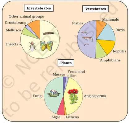
Introduction: This chapter introduces biodiversity — the variety of life at genetic, species and ecosystem levels — and places it in ecological, economic and cultural context. It explains global and Indian patterns of biodiversity, the concept of biodiversity hotspots, and methods used to estimate and compare diversity. Importance: Biodiversity underpins ecosystem services (provisioning, regulating, supporting and cultural), sustains agriculture and medicine, and maintains ecological balance. The chapter highlights why conserving biodiversity is essential for human well‑being, food security and long‑term sustainability. Key themes: - Levels of biodiversity: genetic, species and ecosystem diversity and their interrelationships. - Measuring diversity: species richness, relative abundance and indices (e.g., Simpson's index) and sampling methods. - Global and local patterns: latitudinal gradients, biodiversity hotspots and India’s megadiversity status. - Threats: habitat loss and fragmentation, overexploitation, pollution, invasive species, climate change and genetic erosion. - Conservation strategies: in situ (protected areas, biosphere reserves, wildlife sanctuaries, national…
Learning Objectives
- Define biodiversity and differentiate between genetic, species and ecosystem diversity.
- Explain the ecological, economic and social significance of biodiversity with suitable examples.
- List major causes of biodiversity loss and describe how each threat (habitat loss, overexploitation, invasive species, pollution, climate change) impacts species and ecosystems.
- Identify the characteristics of biodiversity hotspots and name the principal hotspots in India.
- Describe the IUCN categories of threat and interpret Red Data Book entries for given species.
- Compare in-situ and ex-situ conservation methods and give representative examples of each.
- Outline the role and functions of biosphere reserves, national parks and wildlife sanctuaries in biodiversity conservation.
- Explain the importance and working principles of gene banks, seed banks, botanical gardens and cryopreservation in ex-situ conservation.
Topics in this chapter
25 topics · tap a topic title to jump straight to it.
Introduction to biodiversity
Definition: Biodiversity (biological diversity) is the variety and variability of life on Earth. It includes variation at three hierarchical levels: genetic diversity, species diversity and ecosystem diversity.
Levels of biodiversity
- Genetic diversity: Variation of genes within a species (different alleles, populations). Example: different wheat varieties adapted to drought.
- Species diversity: Number and relative abundance of species in an area. It has two components: species richness (count of species) and species evenness (how evenly individuals are distributed).
- Ecosystem diversity: Variety of ecosystems/communities (forests, wetlands, coral reefs, grasslands) and ecological processes.
Why biodiversity matters
- Ecosystem services: Provisioning (food, medicine), regulating (climate, flood control), supporting (nutrient cycling, pollination), cultural (recreation, spiritual).
- Resilience: Diverse systems better resist and recover from disturbances.
- Economic & scientific value: Agriculture, pharmaceuticals, tourism, research.
Threats to biodiversity
- Habitat loss and fragmentation
- Overexploitation (overfishing, hunting)
- Pollution (chemical, plastic, eutrophication)
- Invasive alien species
- Climate change
Measuring biodiversity (concepts)
- Species richness (S): number of species recorded in an area.
- Relative abundance (p_i): proportion of individuals of species i = n_i / N.
- Species-area relationship: larger areas usually contain more species (S = c A^z).
Conservation approaches
- In-situ: Protected areas (national parks, wildlife sanctuaries), biosphere reserves, community conserved areas, sacred groves.
- Ex-situ: Seed banks, botanical gardens, captive breeding, cryopreservation.
- Policy & legal tools: Convention on Biological Diversity (CBD), CITES, national wildlife protection laws.
Notes on hotspots: Biodiversity hotspots are regions with very high endemism and high habitat loss. Typical criteria: at least 1500 endemic vascular plant species and loss of at least 70% of original habitat. Examples include the Western Ghats and Eastern Himalaya.
- Amazon rainforest: extremely high species and ecosystem diversity; important for global climate regulation.
- Coral reefs: high marine biodiversity; threatened by bleaching and ocean acidification.
- Tiger (Panthera tigris) as an umbrella species: protecting tiger habitats conserves many other species.
- Pollinators (bees, butterflies): support agricultural crop production and wild plant reproduction.
- Gut microbiome: genetic and species diversity within humans affects digestion and immunity.
- Agricultural monoculture (e.g., large-scale single-crop fields): reduced biodiversity, greater vulnerability to pests and climate stress.
- Relative abundance: p_i = n_i / N (n_i = individuals of species i; N = total individuals)
- Species-area relationship: S = c * A^z (S = species number; A = area; c and z are constants; z usually 0.1–0.4)
- Simpson's Diversity Index (probability that two randomly chosen individuals belong to same species): λ = Σ(p_i^2). Simpson's Index of Diversity = 1 - λ. Simpson's reciprocal index = 1 / Σ(p_i^2).
- Shannon-Wiener Index: H' = -Σ(p_i * ln p_i) (higher H' = higher diversity)
- Margalef's Richness Index: R = (S - 1) / ln(N) (S = number of species, N = total individuals)
- Pielou's Evenness: J = H' / ln(S) (measures how evenly individuals are distributed among species)
Levels of biodiversity
Biodiversity is the variety of life at all levels — genes, species and ecosystems. In CBSE Class 12 Biology, biodiversity is described in three hierarchical levels: genetic diversity, species diversity and ecosystem diversity. Each level has its own meaning, significance and methods of measurement.
1. Genetic diversity
Genetic diversity is the variation of genes within a species (differences in alleles, gene frequencies and genotypes). It underlies a population’s ability to adapt to changing environments and resist diseases.
- Importance: Enables natural selection and long-term survival; provides raw material for plant and animal breeding.
- Measures & examples: heterozygosity, allelic richness, percent polymorphic loci. Examples include different breeds of dogs, rice varieties (e.g., basmati vs IR varieties) and genetic differences among human populations.
2. Species diversity
Species diversity refers to the variety and abundance of different species in a community. It has two components: species richness (number of species) and species evenness (relative abundances).
- Importance: High species diversity stabilizes ecosystems, supports ecosystem services and increases resilience.
- Measures: species richness (S), Shannon-Wiener index (H'), Simpson’s index, species evenness (E).
3. Ecosystem diversity
Ecosystem diversity is the variety of ecosystems or habitats in a region (forests, grasslands, wetlands, coral reefs, deserts). It includes ecological processes and interactions among communities and their abiotic environment.
- Importance: Different ecosystems provide distinct services (e.g., wetlands purify water, forests regulate climate). Loss of ecosystem diversity reduces available niches and services.
- Examples: tropical rainforests, mangroves, coral reef systems, alpine meadows.
Connections among levels
Genetic variation within species affects species diversity (speciation potential) and ecosystem function; species composition shapes ecosystem processes. Conservation strategies often target all three levels (protected areas for ecosystems, gene banks for genetic diversity, species protection for threatened taxa).
Threats and conservation
Threats include habitat loss, overexploitation, pollution, invasive species and climate change. Conservation approaches: in situ (protected areas, biosphere reserves) and ex situ (seed banks, captive breeding), plus sustainable use and restoration.
Summary
Levels of biodiversity—genetic, species and ecosystem—are nested and interdependent. Measuring and conserving diversity at each level is essential for ecological stability, human welfare and long-term evolution.
- Genetic diversity: Different varieties of rice (e.g., traditional local varieties vs high-yield hybrids) enabling farmers to choose varieties adapted to drought, pests or soil types.
- Genetic diversity (adaptation example): Industrial melanism in the peppered moth (Biston betularia) — allele frequency changed during/after the Industrial Revolution.
- Species diversity: Amazon rainforest and Western Ghats both show very high species richness and endemic species, supporting complex food webs.
- Ecosystem diversity: Sundarbans mangrove ecosystem vs coral reefs — each provides distinct services (coastal protection, nursery grounds vs tourism, fisheries).
- Loss example: Monoculture cropping reduces genetic and species diversity, increasing vulnerability to pests and diseases (e.g., Irish potato famine historical example).
- Relative abundance: p_i = n_i / N (n_i = individuals of species i; N = total individuals)
- Shannon–Wiener index: H' = -Σ p_i ln(p_i) (higher H' = higher diversity)
- Pielou’s evenness: E = H' / ln(S) (S = number of species; 0 < E ≤ 1)
- Simpson’s index: D = 1 - Σ (n_i / N)^2 (value approaches 1 for high diversity; some texts use λ = Σ (n_i/N)^2 as dominance)
- Species–area relationship: S = c A^z (S = species number, A = area, c and z are constants; log form: log S = log c + z log A)
- Beta diversity (species turnover): β = γ / α (α = mean species richness per sample, γ = total species richness across samples)
Genetic diversity
What is genetic diversity?
Genetic diversity (also called genetic variation) is the variation in DNA sequences among individuals within a population and between populations of the same species. It includes differences in alleles, genes, and chromosomes that produce variation in traits. Genetic diversity is the raw material for evolution and adaptation.
Why it matters
- Enables populations to adapt to changing environments (disease, climate, pests).
- Reduces risk of extinction by providing variants that may survive new stresses.
- Supports agriculture and medicine by providing useful alleles (e.g., disease resistance).
Sources of genetic variation
- Mutation — random changes in DNA that create new alleles.
- Sexual recombination — independent assortment and crossing-over that reshuffle alleles.
- Gene flow (migration) — movement of alleles between populations.
- Genetic drift — random changes in allele frequency especially in small populations (founder effect, bottleneck).
- Natural selection — changes allele frequencies by differential survival and reproduction.
Levels of genetic diversity
- Within individuals — heterozygosity (two different alleles at a locus).
- Within populations — allele frequencies and genotype frequencies across members of a population.
- Between populations — differentiation measured by statistics like FST.
Measuring genetic diversity (concepts)
- Allele frequency — proportion of copies of an allele in a population (p, q, etc.).
- Heterozygosity — probability that two alleles randomly chosen from the population are different. Observed heterozygosity (Ho) vs expected heterozygosity (He).
- Genetic differentiation (FST) — fraction of genetic variance among populations relative to total variance; higher FST = more differentiation.
- Effective population size (Ne) — the size of an idealized population that would show the same amount of genetic drift; often lower than census size.
Threats to genetic diversity
- Habitat fragmentation and small isolated populations (increase drift, inbreeding).
- Bottlenecks and founder events (large loss of alleles).
- Overexploitation and selective breeding (loss of wild alleles).
- Pollution and diseases that reduce population size.
Conservation implications
Maintaining genetic diversity is a key objective of conservation. Strategies include preserving large and connected populations, creating gene banks (seeds, gametes), managed breeding programs that avoid inbreeding, and facilitating gene flow (wildlife corridors).
Simple classroom summary
Genetic diversity is the variety of genetic information within and among populations. It arises from mutation and recombination and is shaped by selection, drift and migration. It is essential for adaptability and long-term survival of species.
- Sickle cell anemia and malaria: The sickle-cell allele confers resistance to malaria in heterozygotes (heterozygote advantage maintains genetic variation).
- Peppered moth (Biston betularia): Industrial melanism illustrated selection changing allele frequencies in response to pollution.
- Antibiotic resistance in bacteria: New mutations and selection by antibiotics create resistant strains—rapid change in allele frequencies.
- Cheetahs: Very low genetic diversity due to historic bottlenecks, resulting in high vulnerability to disease and reduced reproductive fitness.
- Crop landraces vs modern varieties: Traditional landraces often hold high genetic diversity useful for breeding, whereas many high-yield cultivars are genetically uniform.
- Tasmanian devil: Low diversity and a transmissible facial tumor highlight risks of reduced genetic variation.
- Allele frequency: p + q = 1 (for a single gene with two alleles)
- Hardy–Weinberg genotype frequencies: p^2 + 2pq + q^2 = 1 (expected genotype proportions when a population is in HW equilibrium)
- Expected heterozygosity (gene diversity): He = 1 - Σ pi^2 (sum over all allele frequencies pi at a locus)
- Observed inbreeding coefficient: F = (He - Ho) / He (Ho = observed heterozygosity, He = expected)
- Effective population size for unequal sex ratio: Ne = (4 * Nm * Nf) / (Nm + Nf) (Nm = number of breeding males, Nf = breeding females)
- Fixation index (genetic differentiation): FST = (HT - HS) / HT (HT = total expected heterozygosity, HS = subpopulation expected heterozygosity)
Species diversity
Definition: Species diversity is the variety and abundance distribution of different species in a defined ecological community or region. It combines two components: species richness (the number of species) and species evenness (how evenly individuals are distributed among those species).
Components:
- Species richness (S): a simple count of species present in the sample or community.
- Species evenness (E): indicates whether the community is dominated by one or few species (low evenness) or whether individuals are more equally distributed (high evenness).
Levels of diversity (spatial scale):
- Alpha (α) diversity: diversity within a single community or habitat (local diversity).
- Beta (β) diversity: turnover in species composition between communities or habitats (connects α and γ).
- Gamma (γ) diversity: total species diversity across a larger region or landscape.
- Common relation (Whittaker): β ≈ γ / α (some definitions use βw = (γ/α) − 1).
Common quantitative indices:
- Shannon–Wiener (Shannon) index: H' = − Σ pi ln(pi), where pi = ni / N (ni = individuals of species i, N = total individuals). Higher H' indicates greater diversity and/or evenness.
- Simpson's index: D = Σ pi^2. Often reported as Simpson's diversity = 1 − D (probability that two randomly chosen individuals belong to different species) or as inverse Simpson 1 / D (larger values = higher diversity).
- Evenness (Pielou's): J = H' / ln(S), ranges from 0 to 1 (1 = complete evenness).
Interpretation and ecological significance: Two communities can have the same species richness but different diversity if one is dominated by a single species (low evenness). High species diversity typically increases ecosystem stability, resilience and productivity. Diversity patterns are influenced by habitat heterogeneity, climate, area, disturbance and evolutionary history.
Sampling and comparability: Indices require careful sampling (same effort, area and method) before comparing communities. Rarefaction and standardized sampling are used to correct for unequal sample sizes.
Conservation relevance: Areas with high species diversity (e.g., tropical rainforests, coral reefs) are conservation priorities. Loss of species or evenness (e.g., from invasive species or monoculture agriculture) reduces ecosystem services and resilience.
- Tropical rainforests: very high species richness and often high evenness — many tree, insect and bird species share resources; example: Amazon rainforest.
- Desert ecosystems: low species richness, often dominated by a few well-adapted species (low evenness).
- Coral reefs: extremely high species diversity (many fish, corals, invertebrates) — considered biodiversity hotspots.
- Agricultural monoculture (e.g., large wheat field): very low species diversity compared with adjacent natural grassland.
- Island biogeography: small or isolated islands often have lower species richness; species turnover and endemism illustrate beta and gamma diversity (e.g., Galápagos).
- Invasive species example: Introduction of Nile perch in Lake Victoria reduced native cichlid diversity (loss of species richness and evenness).
- Species richness: S = number of species in the sample or community.
- Relative abundance: pi = ni / N (ni = individuals of species i, N = total individuals of all species).
- Shannon–Wiener index: H' = - Σ (pi * ln pi) (sum over all species).
- Pielou's evenness: J = H' / ln(S) (0 ≤ J ≤ 1).
- Simpson's index: D = Σ (pi^2). Simpson's diversity = 1 - D (or inverse Simpson = 1 / D).
- Species–area relationship: S = c * A^z (or log S = z * log A + log c), where A = area, c and z are constants.
Ecosystem diversity
Definition: Ecosystem diversity is the variety of ecosystems in a given region or on the Earth as a whole. It includes the range of different habitats, biological communities, ecological processes and interactions between organisms and their physical environment.
Main components:
- Habitat diversity: different physical environments (forests, wetlands, grasslands, deserts, coral reefs, etc.).
- Community diversity: different assemblages of species and their food webs and interactions in each habitat.
- Ecological processes: energy flow, nutrient cycling, succession, disturbance regimes and hydrological regimes that differ among ecosystems.
Why it matters: High ecosystem diversity increases overall biodiversity (by providing many niches), supports a wide range of ecosystem services (food, water purification, climate regulation, pollination), improves resilience to disturbances (disease, climate change) and supplies cultural and economic benefits.
Measurement and relationships: Ecosystem diversity is often described qualitatively (types and extent of ecosystems) and quantitatively via surrogates such as the number of ecosystem types, area occupied, landscape heterogeneity, and turnover of species among habitats (beta diversity). Ecosystem diversity interacts with species and genetic diversity: loss of ecosystems causes declines in species and genetic diversity.
Threats and conservation: Major threats include habitat destruction and fragmentation, land-use change (agriculture, urbanization), pollution, invasive species, overexploitation and climate change. Conservation actions include protected-area networks covering representative ecosystems, restoration ecology, landscape-level planning (ecological corridors), sustainable resource management and policies to maintain ecosystem processes.
- Tropical rainforest mosaic: multi-layered canopy, diverse animal and plant communities, high productivity and many microhabitats.
- Coral reef ecosystems: high structural complexity, numerous niches for fish, corals and invertebrates; provide coastal protection and fisheries.
- Mangrove swamps: intertidal ecosystems that trap sediments, protect coasts, and act as nurseries for fish and crustaceans.
- Alpine and montane ecosystems: altitude-driven variation in vegetation zones, endemic species, distinct hydrology.
- Agricultural monoculture vs mixed agroforestry: monocultures represent low ecosystem diversity and reduced services; agroforestry increases habitat diversity and resilience.
- Urban ecosystems: novel assemblages of species adapted to built environments; green roofs, parks and riparian corridors increase urban ecosystem diversity.
- Species–area relationship: S = c * A^z (S = number of species, A = area, c and z are constants; in log form: log S = log c + z log A). Useful to relate area of ecosystems to expected species richness.
- Shannon–Wiener index (for diversity within an ecosystem): H' = -Σ (p_i * ln p_i) (p_i = proportion of individuals of species i).
- Simpson's index (dominance): D = Σ p_i^2 ; Simpson's diversity = 1 - D (higher values = greater diversity).
- Evenness (Pielou's index): J' = H' / ln(S) (S = number of species; measures how equal abundances are).
- Beta diversity (turnover between ecosystems): multiplicative form β = γ / α (γ = total regional species richness, α = average local richness); additive form β = γ - α.
- Sørensen similarity index (between two ecosystems): QS = 2C / (S1 + S2) (C = number of common species, S1 and S2 = species counts in each ecosystem).
Levels of biodiversity organisation (global, national, local)
Overview: Biodiversity can be studied at different spatial scales — global, national and local. Each level highlights different components (genetic, species, ecosystem) and requires different measurement methods and conservation approaches. Scale matters: processes that shape diversity (evolution, speciation, habitat heterogeneity, human impacts) operate differently at each level.
Global level
Definition: Patterns and amounts of biodiversity across the Earth (all species, ecosystems and their genetic variation). Key concepts include biogeographic realms, biodiversity hotspots, latitudinal gradients and global endemism.
- What is measured: total number of species (global species richness estimate), distribution of major ecosystems, global endemism, large-scale genetic lineages.
- Important patterns: latitudinal diversity gradient (more species in the tropics), species–area relationship at continental scales, centers of endemism and hotspots (regions with high endemism and high threat).
- Conservation implication: international agreements (CBD, CITES), global monitoring, transboundary protected areas.
National level
Definition: Biodiversity within a country's political boundaries — species lists, endemics, ecosystems and protected-area networks of that nation.
- What is measured: national species inventories, red lists of threatened species, ecosystem mapping, genetic resources important to the country (crop landraces, livestock breeds).
- Important considerations: national endemics, design and management of protected areas (national parks, wildlife sanctuaries), biodiversity laws and policy.
- Conservation implication: national strategies, reserve networks, ex situ conservation (seed banks), sustainable use policies.
Local level
Definition: Diversity at the scale of a habitat, community or site (e.g., a forest patch, pond, school campus).
- What is measured: alpha diversity (species richness/heterogeneity within a site), species composition, relative abundances, functional groups and genetic variation within local populations.
- Important measures and comparisons: alpha (within-site), beta (between-site turnover), gamma (landscape or region total) diversity — used to understand small-scale heterogeneity and management needs.
- Conservation implication: local habitat management, restoration, control of invasive species, community-based conservation.
Linking levels
Local diversity (alpha) aggregated across sites makes regional (gamma) diversity; differences among sites (beta) determine how many unique species are contributed. Protecting diversity requires action at all scales — local management, national policy and international cooperation.
Measurement notes: Different indices capture richness and evenness. Sampling design matters (plot size, effort) because species counts increase with sampled area and effort (species–area relationship and species accumulation curves).
Teaching tip: Emphasize scale dependence with examples: a small meadow may have high local (alpha) plant diversity, but the country’s unique species (endemics) determine national conservation priorities.
- Global — Coral Triangle (Southeast Asia): world’s highest marine species richness; Amazon rainforest: very high terrestrial species richness and global endemism.
- Global — Latitudinal gradient: tropical rainforests (equator) vs tundra (high latitudes) — species richness decreases with latitude.
- National (India) — Western Ghats and Eastern Himalaya: centres of endemism; Sunderbans: unique mangrove ecosystem.
- National — Agricultural crop diversity: India’s many traditional rice landraces vs modern monoculture varieties (shows national genetic resource issues).
- Local — A village pond: macroinvertebrate and aquatic plant species composition; a school campus: count of tree species (alpha diversity).
- Local — Two neighbouring forest patches: different tree species composition (beta diversity) contributing to the landscape (gamma) diversity.
- Species–area relationship: S = c A^z, where S = number of species, A = area, c and z are constants (log form: log S = log c + z log A).
- Shannon (Wiener) diversity index: H' = -Σ (p_i ln p_i), where p_i = proportion of individuals of species i. Higher H' = higher diversity.
- Pielou’s evenness: J' = H' / ln(S), where S = species richness (number of species).
- Simpson’s index (probability that two individuals randomly selected are of same species): D = Σ [n_i (n_i - 1)] / [N (N - 1)]. Commonly reported as 1 - D or 1/D (Simpson’s reciprocal) to express diversity positively.
- Whittaker’s beta diversity (one common form): β_W = γ / α, where γ = total species in landscape and α = mean species per site. (Alternative formulation: β = (γ/α) - 1.)
- Jaccard similarity index (between two sites): J = c / (a + b - c), where a = species in site A, b = species in site B, c = species common to both.
Biodiversity hotspots
Definition: Biodiversity hotspots are regions that contain exceptional concentrations of endemic species and are experiencing exceptional loss of habitat. The concept (proposed by Norman Myers) is used to prioritize areas for conservation.
- Formal criteria: A region qualifies as a hotspot if (1) it contains at least 1,500 species of vascular plants (> 0.5% of the world’s total) as endemics, and (2) it has lost at least 70% of its original native vegetation.
- Why hotspots matter: Although hotspots cover a small fraction of Earth’s land surface, they harbor a large proportion of the world’s terrestrial biodiversity (high species richness and endemism) and many threatened species — so protecting them yields a high conservation return on effort.
- Characteristics of hotspots:
- High species richness and high level of endemism
- Complex topography and a variety of microclimates
- Evolutionary history that promoted speciation (isolation, refugia, ancient stable climates)
- Strong human pressure: habitat conversion, fragmentation and other threats
- Main threats: Habitat destruction and fragmentation (agriculture, urbanization), invasive alien species, overexploitation, pollution, and climate change.
- Conservation approaches:
- Protected areas (national parks, wildlife sanctuaries) and ecological corridors to reduce fragmentation
- Habitat restoration and reforestation
- In-situ conservation (community-conserved areas) and ex-situ methods (botanical gardens, seed banks)
- Legal protection, sustainable resource-use policies and community engagement
- Prioritization using hotspot criteria to allocate limited conservation resources
- Global context: As of standard hotspot assessments, there are a set of internationally recognized hotspots (commonly cited number: 34). They occupy a small percentage of land area but support a disproportionately large share of plant and animal diversity, making them key targets for conservation.
CBSE relevance: In Class 12 Biology (Biodiversity and Conservation), hotspots illustrate how scientists identify priority areas for biodiversity protection and the importance of focusing conservation efforts where they will protect the most endemic and threatened species.
- Western Ghats (India): High plant endemism, many endemic amphibians and mammals; heavily impacted by agriculture and development — designated a global hotspot.
- Eastern Himalaya (India, Nepal, Bhutan, Myanmar): Extremely high species richness and endemism across altitudinal zones; threatened by deforestation and habitat fragmentation.
- Indo-Burma (Northeast India, Myanmar, Thailand, Vietnam): Rich in endemic plants and freshwater fishes; faces habitat loss from agriculture and urban expansion.
- Sundaland (Malay Peninsula, Borneo, Sumatra, Java): Tropical rainforests with many endemic species; deforestation for oil palm is a major threat.
- Mediterranean Basin: High plant endemism adapted to seasonal climates; threatened by urbanization, agriculture and invasive species.
- Madagascar and the Indian Ocean islands: Extremely high levels of unique flora and fauna (e.g., lemurs); habitat destruction and introduced species are major threats.
- Species richness (S): simple count of species in an area (no complex formula).
- Species–area relationship (Arrhenius): S = c * A^z (S = number of species, A = area, c and z are constants).
- Log form of species–area: log S = log c + z log A (useful for plotting on log–log graphs).
- Shannon diversity index: H' = -Σ (p_i * ln p_i) (p_i = proportion of individuals in species i; higher H' means greater diversity).
- Simpson’s diversity index (probability form): D = 1 - Σ (p_i^2) (values range from 0 to 1; higher = more diversity).
- Evenness (Pielou's): J = H' / ln(S) (measures how equal the abundances of species are).
Values of biodiversity
Values of biodiversity
Biodiversity is the variety of life at genetic, species and ecosystem levels. Its values are the benefits that humans obtain directly or indirectly from biological diversity. These values can be economic, ecological, social, cultural and ethical. Recognising these values helps justify conservation and sustainable use.
Major categories of values
- Provisioning (direct use) values: Tangible products obtained from ecosystems such as food, timber, fuel, fibres, fresh water, medicines and genetic material for crop and livestock improvement.
- Regulating (indirect) values: Ecosystem processes that regulate climate, diseases, floods, water purification, pollination and erosion control that maintain environmental stability.
- Supporting (ecological) values: Fundamental services such as primary production, nutrient cycling, soil formation and habitat provision that enable other ecosystem services.
- Cultural values: Non-material benefits like recreational, spiritual, educational and aesthetic values (eco-tourism, sacred groves).
- Option and existence values: Option value is the potential of biodiversity to provide future benefits (new drugs, crops). Existence value is the value people place on knowing a species or ecosystem exists even if they never use it.
- Ethical and intrinsic values: The moral responsibility to protect other species and ecosystems irrespective of human use.
Why these values matter
1) Lifeline for humans: Provisioning services supply food, fibres, medicines and raw materials. 2) Risk reduction: Regulating services reduce flood damage, disease outbreaks and climate extremes. 3) Economic foundation: Many industries (agriculture, pharmaceuticals, forestry, fisheries, tourism) depend on biodiversity. 4) Genetic resources: Wild relatives of crops and livestock provide genes for resistance and improved traits. 5) Resilience: Diverse ecosystems recover better from disturbances and maintain long-term productivity.
Examples linking value and consequence
- Pollination by bees and other insects supports fruit and seed production for many crops; pollinator loss reduces yields and farm incomes.
- Mangrove forests protect coasts from storms and reduce erosion; their removal increases coastal damage and economic loss.
- Wild plants (e.g., rosy periwinkle) yielded anti-cancer alkaloids; many medicines are derived from plant and microbial metabolites.
- Overfishing reduces fish stocks and collapses fisheries, demonstrating loss of provisioning value when biodiversity is not managed.
Valuation concepts
Economic valuation groups values into Use values (direct and indirect), Option value, and Non-use (existence/heritage) value. Total Economic Value (TEV) is often expressed as the sum of these components and is used in policy and cost–benefit analyses to justify conservation.
Conservation implication: Because many ecological services are not priced in markets, biodiversity is often undervalued. Recognising and accounting for all values encourages sustainable management and policy measures such as protected areas, payment for ecosystem services and habitat restoration.
- Pollination: Bees and butterflies pollinate crops such as apples, almonds and cotton; decline in pollinators lowers crop yields.
- Medicinal plants: Rosy periwinkle provided vincristine and vinblastine used in cancer treatment; aspirin originally derived from willow bark.
- Coastal protection: Mangroves and coral reefs reduce wave energy and protect shorelines during storms.
- Genetic improvement: Wild relatives of wheat, rice or maize supply genes for pest resistance and drought tolerance used in breeding.
- Fisheries and livelihoods: Coastal and inland fish biodiversity supports food security and incomes; overexploitation leads to fishery collapse.
- Species richness: S = total number of species in a sample or area.
- Relative abundance: p_i = n_i / N (where n_i is individuals of species i, N is total individuals).
- Shannon-Wiener index: H' = -Σ(p_i ln p_i), measures diversity combining richness and evenness.
- Simpson's index of diversity: D = 1 - Σ[n_i(n_i - 1)] / [N(N - 1)], higher D means greater diversity.
- Evenness: E = H' / ln(S), ranges 0–1; 1 indicates complete evenness among species.
- Total Economic Value (conceptual): TEV = Use values + Option value + Non-use (existence/cultural) values.
Threats to biodiversity
Overview
Biodiversity (variety of life at genetic, species and ecosystem levels) is threatened by multiple, often interacting, processes—mostly driven by human activities. Loss of biodiversity reduces ecosystem services, resilience and evolutionary potential.
Main threats (with mechanisms)
- Habitat loss and fragmentation: Conversion of forests, wetlands and grasslands to agriculture, urban areas, roads and dams removes or isolates populations. Fragmentation reduces patch size, increases edge effects and limits movement, resulting in local extinctions.
- Overexploitation: Unsustainable hunting, fishing and harvesting (timber, non-timber forest products) reduce population sizes below recovery thresholds (e.g., overfishing of cod; ivory-driven elephant declines).
- Invasive alien species: Non-native plants, animals or pathogens can outcompete, prey on or bring diseases to native species (e.g., Nile perch in Lake Victoria, water hyacinth clogging waterways).
- Pollution: Pesticides, heavy metals, plastics, nutrient runoff and oil spills degrade habitats and cause direct mortality or sublethal effects (e.g., DDT causing eggshell thinning in raptors; eutrophication causing dead zones).
- Climate change: Altered temperature/precipitation patterns, sea-level rise and increased extreme events shift species ranges, phenology and cause coral bleaching and loss of ice-dependent species (e.g., polar bears, coral reefs).
- Diseases: Emergent pathogens can cause rapid population declines (e.g., chytrid fungus in amphibians, chestnut blight).
- Small population effects: Genetic drift, inbreeding depression, loss of genetic variability and Allee effects reduce fitness and increase extinction risk for small populations.
- Co-extinction: Loss of one species (host or mutualist) can cause dependent species to disappear (e.g., specialist parasites or pollinators).
Interaction and cumulative effects
Threats commonly act together (e.g., climate change amplifies habitat loss effects; invasive species exploit disturbed habitats). This makes predicting outcomes complex and accelerates biodiversity loss.
Consequences
- Reduced ecosystem services (pollination, water purification, soil fertility)
- Loss of genetic resources and potential medicines
- Increased vulnerability of ecosystems to disturbance
- Irreversible extinctions and loss of evolutionary history
Conservation implications (brief)
Addressing threats requires habitat protection and restoration, sustainable use, control of invasives, pollution reduction, disease monitoring, climate mitigation/adaptation and maintaining sufficiently large, connected populations (protected area networks, corridors, ex situ conservation where necessary).
- Deforestation in the Amazon reducing habitat for innumerable species and fragmenting populations.
- Collapse of Atlantic cod fisheries in the late 20th century due to overfishing; long recovery times.
- Nile perch introduction in Lake Victoria causing extinction of many native cichlid species.
- Water hyacinth (Eichhornia crassipes) choking Indian lakes and canals, reducing native aquatic biodiversity.
- DDT use historically caused eggshell thinning and declines in raptors (e.g., peregrine falcon); recovery followed DDT bans and conservation.
- Coral bleaching events on the Great Barrier Reef caused by ocean warming and mass coral mortality.
- Species–area relationship: S = c A^z (S = number of species, A = area, c and z are constants). Log form: log S = log c + z log A. Useful to estimate species loss from habitat area reduction.
- Shannon–Wiener index: H' = -Σ (p_i * ln p_i) (p_i = proportion of individuals of species i). Measures species diversity accounting for abundance and richness.
- Simpson's index (probability two randomly chosen individuals are same species): D = Σ [n_i (n_i - 1)] / [N (N - 1)]. Simpson's diversity = 1 - D (higher = more diverse).
- Effective population size (diploid): N_e = (4 N_m N_f) / (N_m + N_f) (N_m and N_f = number of breeding males and females). Determines rate of genetic drift and inbreeding.
- Loss of heterozygosity per generation ≈ 1 / (2 N_e). Inbreeding coefficient change per generation ΔF ≈ 1 / (2 N_e). Small N_e → faster genetic diversity loss.
Endemic, endangered and extinct species
Definitions
- Endemic species: Species native to and restricted to a specific geographic area (island, mountain range, country or habitat). They are not naturally found anywhere else.
- Endangered species: Species facing a very high risk of extinction in the wild in the near future. This is an IUCN threat category (examples: Endangered, Critically Endangered).
- Extinct species: Species for which there is no reasonable doubt that the last individual has died. (IUCN category: Extinct).
Key distinctions
- Endemic refers to geographic restriction; it does not necessarily imply a threatened status (though endemics are more vulnerable to threats).
- Endangered is a risk status based on population trends, range, and other criteria. An endemic species can be endangered, but not all endangered species are endemic.
- Extinct is the final outcome when threats are not reversed; extinct species are no longer present on Earth.
Causes of endangerment and extinction
- Habitat loss and fragmentation (deforestation, land conversion, dams, urbanisation).
- Overexploitation (hunting, fishing, logging).
- Invasive alien species and diseases.
- Pollution (chemical, plastic, eutrophication).
- Climate change (range shifts, altered phenology, extreme events).
- Small population size, genetic drift, inbreeding and stochastic events.
IUCN categories (summary)
- Least Concern (LC), Near Threatened (NT), Vulnerable (VU), Endangered (EN), Critically Endangered (CR), Extinct in the Wild (EW), Extinct (EX).
Conservation approaches
- In situ conservation: Protected areas (national parks, sanctuaries, biosphere reserves), habitat restoration, wildlife corridors and community-managed conservation.
- Ex situ conservation: Zoos and aquaria, botanical gardens, seed banks, cryopreservation, captive breeding and reintroduction programs.
- Legal protection (national laws, CITES), species recovery plans, awareness and community involvement, controlling invasive species and reducing poaching.
Why endemics are important
- High conservation priority because loss of an endemic species means global extinction.
- Often adapted to local ecological roles; their loss can destabilise ecosystems.
Class 12 relevance and examples
- Use endemic, endangered and extinct species as case studies to understand biodiversity loss and conservation planning.
- Compare population trends, causes and conservation responses across examples.
- Endemic: Lion-tailed macaque (Macaca silenus) — endemic to Western Ghats (India); highly restricted range and threatened by habitat fragmentation.
- Endemic: Madagascar lemurs (multiple species) — endemic to Madagascar; many species are threatened due to deforestation.
- Endangered: Bengal tiger (Panthera tigris tigris) — listed as Endangered; threats include habitat loss and poaching.
- Endangered / Critically Endangered: Gharial (Gavialis gangeticus) — critically endangered due to river habitat degradation and fishing nets.
- Extinct: Dodo (Raphus cucullatus) — extinct in late 17th century following hunting and introduced species on Mauritius.
- Extinct: Passenger pigeon (Ectopistes migratorius) — once abundant in North America; hunted to extinction in early 20th century.
- Species–area relationship: S = c * A^z (S = number of species, A = area, c and z are constants). Often plotted as log S = log c + z log A.
- Effective population size (diploid): Ne = (4 * Nm * Nf) / (Nm + Nf) (Nm = number of breeding males, Nf = number of breeding females).
- Rate of inbreeding (approximate): ΔF ≈ 1 / (2 * Ne) per generation (increase in inbreeding coefficient per generation).
- Heterozygosity loss (approx): Ht ≈ H0 * (1 - 1/(2Ne))^t (Ht = heterozygosity after t generations).
- Shannon index (diversity): H' = -Σ (p_i * ln p_i) (p_i = proportion of individuals in species i).
- Simpson's index (diversity): D = 1 - Σ [n_i (n_i - 1)] / [N (N - 1)] (n_i = number of individuals of species i, N = total individuals).
Conservation — concepts and objectives
Definition: Conservation is the planned management of natural resources (biological diversity, ecosystems and genetic resources) to sustain their availability and functioning for present and future generations while allowing sustainable use. It balances protection, sustainable use and restoration.
Core concepts
- Biodiversity levels: genetic diversity (variation within species), species diversity (number and relative abundance of species) and ecosystem diversity (variety of habitats and ecological processes).
- In situ conservation: conserving species in their natural habitats — protected areas (national parks, wildlife sanctuaries, biosphere reserves), community conserved areas and habitat management.
- Ex situ conservation: conservation outside natural habitats — seed banks, gene banks, botanical gardens, captive breeding, cryopreservation.
- Hotspots and endemism: regions with high species richness and endemism under threat are priority areas for conservation.
- Keystone, umbrella and flagship species: keystone species have disproportionate ecosystem effects; umbrella species protect many others when conserved; flagship species attract public support.
- Metapopulation concept: populations exist as a network of subpopulations with migration; connectivity between patches matters for persistence.
Objectives of conservation
- Maintain ecosystem services: conserve processes such as nutrient cycling, pollination, water purification and soil formation that support human well‑being.
- Preserve genetic diversity: retain variation for adaptability and crop/animal breeding, and to reduce inbreeding and extinction risk.
- Protect species and habitats: prevent extinction, recover endangered species and protect representative ecosystems and rare/endemic habitats.
- Ensure sustainable use: use biological resources in ways that do not deplete them — sustainable fisheries, forestry and agro-biodiversity management.
- Restore degraded ecosystems: ecological restoration and rehabilitation to recover functions and native biodiversity.
- Promote equity and livelihoods: integrate local communities, traditional knowledge and benefit-sharing to make conservation socially sustainable.
- Reduce threats: address habitat loss and fragmentation, overexploitation, pollution, invasive species and climate change.
- Monitoring and research: assess biodiversity status, population trends and effectiveness of conservation measures (using indices and long-term data).
Principles and tools
- Landscape-level and ecosystem approaches (connectivity, buffer zones, corridors).
- Precautionary approach: act to prevent harm even when full scientific certainty is lacking.
- Use of quantitative tools: diversity indices, species–area relationships, population viability analysis (PVA), effective population size calculations.
- Legal and policy instruments: protected area networks, CITES, national laws, community forest management and incentive mechanisms (payments for ecosystem services).
Summary: Conservation aims to sustain biodiversity and ecosystem functioning by protecting species and habitats, preserving genetic variation, enabling sustainable use, restoring damaged systems and integrating people’s needs. It uses both in situ and ex situ methods and quantitative tools to guide priorities and measure success.
- Project Tiger (India): creation of protected reserves and management to recover tiger populations in several reserves (e.g., Ranthambhore, Corbett).
- Svalbard Global Seed Vault (Norway): ex situ backup of crop seeds to preserve genetic diversity for global food security.
- Chipko Movement (India): community-led forest protection that slowed deforestation and promoted local stewardship.
- Gir National Park (India): successful in situ conservation that saved and increased the Asiatic lion population.
- Keoladeo National Park (Bharatpur): wetland protection for migratory birds, demonstrating habitat protection’s role in species conservation.
- Coral reef restoration (e.g., reef transplanting and artificial reefs): active restoration to recover reef structure and biodiversity.
- Species–area relationship: S = c A^z (S = number of species, A = area, c and z are constants). Log form: log S = log c + z log A (used to predict species loss with area reduction).
- Shannon diversity index: H' = -Σ (pi ln pi) where pi is the proportion of individuals of species i (measures species diversity considering richness and evenness).
- Simpson's diversity index: D = 1 - Σ (pi^2) (probability that two randomly chosen individuals belong to different species).
- Effective population size (unequal sexes): Ne = (4 Nm Nf) / (Nm + Nf) where Nm and Nf are numbers of breeding males and females (Ne affects genetic drift and inbreeding).
In-situ conservation
Definition: In-situ conservation is the conservation of species in their natural habitats — protecting ecosystems and natural populations so that species can continue evolving under natural selection.
Objectives:
- Protect whole ecosystems and ecological processes.
- Maintain viable populations and natural genetic diversity.
- Allow species to adapt and evolve in response to environmental changes.
Methods and approaches:
- Protected areas: National parks, wildlife sanctuaries, biosphere reserves, conservation reserves and community reserves — legally managed to preserve habitat and species.
- Biosphere reserves: Zonation with core (strict protection), buffer (research/limited use) and transition (sustainable development) areas.
- Habitat management: Fire control, invasive species control, water management, restoration of degraded areas, corridors to reduce fragmentation.
- Species-specific in-situ programmes: Protection of nesting sites, anti-poaching patrols, monitoring and reintroduction within natural ranges.
- Community-based conservation: Sacred groves, community forests and participatory management where local people are stewards.
Key features that make in-situ effective: preserves ecological interactions (predator–prey, pollinators, nutrient cycles), promotes natural selection and behaviour, preserves co-evolved species assemblages and provides larger areas for viable populations.
Advantages: long-term maintenance of ecosystems, supports ecosystem services, allows natural evolutionary processes, often more cost-effective for many species, benefits local communities.
Limitations / challenges: requires large continuous habitat (hard with fragmentation), human–wildlife conflict, enforcement/management costs, may not save very small or critically endangered populations without additional measures (ex-situ or genetic rescue).
Management & policy elements: legal protection, scientific monitoring (population size, genetic diversity, habitat quality), habitat connectivity (corridors), stakeholder engagement and adaptive management plans.
Relation to other concepts: In-situ is complementary to ex-situ conservation (zoos, seed banks). For many species, combination of in-situ protection and targeted ex-situ measures (for very small populations) is optimal.
- Gir National Park (Gujarat, India) — in-situ protection of the Asiatic lion (Panthera leo persica).
- Kaziranga National Park (Assam, India) — protection leading to recovery of the Indian one-horned rhinoceros (Rhinoceros unicornis).
- Sundarbans (India/Bangladesh) — mangrove ecosystem protecting the Bengal tiger and coastal biodiversity.
- Nilgiri Biosphere Reserve (India) — zonation model conserving multiple habitats and endemic species (Western Ghats).
- Great Barrier Reef Marine Park (Australia) — marine in-situ conservation of coral reef ecosystems.
- Sacred groves and community reserves (various parts of India) — community-led protection of small but biodiverse forest patches.
- Species–area relationship: S = c A^z (S = number of species, A = area, c and z are constants). Log form: log S = log c + z log A. Typical z ≈ 0.15–0.35.
- Percent area protected: %Protected = (Area_protected / Total_area) × 100
- Effective population size (sex-structured): Ne = (4 × Nm × Nf) / (Nm + Nf) (Nm = number of breeding males, Nf = number of breeding females).
- Loss of heterozygosity by genetic drift (approx.): Ht = H0 × (1 - 1/(2Ne))^t (Ht = heterozygosity after t generations; Ne = effective population size).
Protected areas and examples
What are protected areas?
Protected areas are clearly defined geographical spaces dedicated and managed through legal or other effective means to achieve long‑term conservation of nature with associated ecosystem services and cultural values. They are the main in‑situ strategy for biodiversity conservation.
Objectives
- Protect native species and their habitats
- Maintain viable populations and ecological processes
- Prevent habitat loss, over‑exploitation and poaching
- Support scientific research, education and sustainable use in buffer/transition zones
Main categories (Indian & international context)
- Biosphere reserves — large areas conserving landscapes, ecosystems, species and genetic variation; follow core–buffer–transition zoning; part of UNESCO’s Man and Biosphere (MAB) programme.
- National parks — strictly protected areas for conservation, public entry regulated; primary objective is protection of ecosystem and biodiversity.
- Wildlife sanctuaries — protect particular species/habitats; some regulated human activities may be permitted.
- Reserved and protected forests — managed under forest laws for protection and sustainable use.
- Community/conservation reserves & sacred groves — locally conserved areas, often managed by communities with traditional rules.
- IUCN categories — I–VI scheme classifying PAs by management objectives (strict nature reserve to sustainable use areas).
Design and management principles
- Size matters: larger reserves generally support more species and larger viable populations.
- Connectivity and corridors reduce isolation and genetic bottlenecks.
- Core–buffer–transition zoning (especially in biosphere reserves) balances strict protection and sustainable human use.
- Mitigate edge effects, control invasive species, anti‑poaching, habitat restoration and monitoring.
Threats: habitat fragmentation, poaching, invasive species, pollution, climate change, human‑wildlife conflict.
Legal & policy instruments (India): Wildlife Protection Act 1972, Forest (Conservation) Act 1980, Project Tiger, Project Elephant, Biosphere Reserve declarations under MAB.
Why protected areas are crucial: They conserve species and ecosystems in situ, maintain ecosystem services (water, soil, pollination), act as reference sites for science and education, and support livelihoods when managed with communities in buffers and transition areas.
- Biosphere reserves: Nilgiri (Western Ghats), Nanda Devi (Uttarakhand), Sundarbans (mangrove, West Bengal), Gulf of Mannar (marine, Tamil Nadu), Manipur (Keibul Lamjao in Loktak surrounds).
- National parks: Jim Corbett (Uttarakhand), Kaziranga (Assam), Ranthambore (Rajasthan), Gir (Gujarat), Bandipur (Karnataka), Sundarbans National Park (West Bengal).
- Wildlife sanctuaries: Bharatpur/Keoladeo (Rajasthan), Ranganathittu (Karnataka), Periyar (Kerala), Manas Wildlife Sanctuary (Assam).
- Community and traditional sites: Sacred groves in Meghalaya and Karnataka; community conserved areas in northeastern India.
- Species–area relationship: S = c A^z (S = number of species, A = area, c = constant, z = slope exponent).
- Log form: log S = log c + z log A (useful for plotting a straight line on log–log axes).
- Proportional loss/gain: S2/S1 = (A2/A1)^z (predicts fraction of species retained when area changes).
- Typical z values: 0.15–0.35 (continental values ≈0.15–0.2; island/fragment values higher ≈0.25–0.35).
Biosphere reserves and Man and Biosphere (MAB)
Biosphere reserves are protected areas meant to conserve biological diversity, maintain ecosystem services and cultural values, and promote sustainable development in ways that are scientifically and socially sound. They are designated under UNESCO's Man and the Biosphere (MAB) Programme (established 1971) and form the World Network of Biosphere Reserves.
Aims of the MAB Programme
- Conserve genetic resources, species and ecosystems.
- Foster sustainable economic and human development.
- Support research, monitoring, education and information exchange about the environment and human interactions with it.
Zonation (core–buffer–transition model)
- Core zone: Strictly protected area for long-term conservation of landscapes, ecosystems, species and genetic variation. Minimal human interference; research and monitoring allowed under strict control.
- Buffer zone: Surrounds or adjoins the core; activities compatible with conservation are allowed (environmental education, recreation, research, limited resource use).
- Transition (or cooperation) zone: Outermost area where sustainable economic and human activities are promoted (agriculture, settlements, resource harvesting) with community involvement.
Functions and activities
- Conservation: Protect representative ecosystems and endangered species, maintain ecological processes.
- Development: Demonstrate sustainable resource management and livelihoods for local communities.
- Logistic support: Conduct research, environmental monitoring, education, training and data exchange.
Key principles of management
- Use of zonation to balance protection and use.
- Adaptive, science-based management and long-term monitoring.
- Involvement of local communities and respect for traditional knowledge.
- Integration of conservation with sustainable development goals.
- Networking and knowledge sharing through the UNESCO World Network of Biosphere Reserves.
Benefits
- Protects biodiversity and ecosystem services (water regulation, soil conservation, pollination).
- Promotes sustainable livelihoods and ecotourism for local people.
- Provides sites for long-term ecological research and environmental education.
- Facilitates international collaboration and technology transfer.
Challenges
- Conflict between conservation goals and local economic pressures.
- Insufficient funding, weak governance or poor enforcement.
- Habitat fragmentation, invasive species and climate change impacts.
- Need for meaningful participation of indigenous and local communities.
How biosphere reserves fit into conservation strategy
Biosphere reserves act as integrated landscape-level models that combine strict protection with zones of sustainable use, linking in-situ conservation with human development needs. They complement national parks, wildlife sanctuaries and other protected areas by providing socio-ecological demonstration sites and scientific monitoring platforms.
- Nilgiri Biosphere Reserve (southern India) – montane forests, high biodiversity and tribal communities; demonstrates landscape-level conservation with tea/coffee agroforestry in transition zones.
- Nanda Devi Biosphere Reserve (Uttarakhand) – alpine and subalpine ecosystems protecting endemic Himalayan flora and fauna; high-value core areas with restricted access.
- Sundarbans Biosphere Reserve (West Bengal/Bangladesh) – mangrove ecosystem protecting the Bengal tiger and providing storm protection and fisheries; example of coastal zone management.
- Gulf of Mannar Biosphere Reserve (Tamil Nadu) – coastal and marine biodiversity, coral reefs, seagrass beds; integrates fisheries management and coastal livelihoods.
- Manas Biosphere Reserve (Assam) – grassland and tropical forest ecosystem with endangered species; example of community involvement in conservation.
- Great Nicobar Biosphere Reserve – island ecosystems with unique endemic species and sensitivity to human impacts.
- Species–area relationship: S = c * A^z (S = number of species, A = area, c and z are constants) — shows how species richness increases with area.
- Shannon diversity index: H' = -Σ (p_i * ln p_i) (p_i = proportion of individuals of species i) — measures species diversity (richness and evenness).
- Simpson's diversity index (dominance): D = Σ p_i^2 (often reported as 1 - D or 1/D to express diversity) — probability that two randomly chosen individuals belong to the same species.
- Logistic population growth (relevance to managing populations inside reserves): dN/dt = rN(1 - N/K) (N = population size, r = intrinsic growth rate, K = carrying capacity).
Ex-situ conservation
Definition: Ex-situ conservation means conserving components of biological diversity outside their natural habitats. It involves maintaining and breeding species, storing seeds, tissues or genetic material in controlled environments (zoos, botanical gardens, seed banks, cryopreservation facilities, etc.) to reduce extinction risk, preserve genetic diversity and enable future reintroduction.
Objectives:
- Safeguard threatened species and their genetic material when in-situ protection is inadequate.
- Maintain living populations for research, education and public awareness.
- Produce individuals for reintroduction or population reinforcement.
- Preserve plant germplasm (seeds, tissue cultures) and microbial strains for agriculture, medicine and restoration.
Major methods:
- Zoos and captive breeding: maintain and breed animals under human care; manage pedigrees to minimise inbreeding and retain genetic diversity.
- Botanical gardens and arboreta: grow and conserve living plants, propagate rare species and provide material for restoration.
- Seed banks and seed storage: store orthodox seeds at low temperature and moisture to extend viability (e.g., Svalbard Global Seed Vault, Millennium Seed Bank).
- Cryopreservation and frozen zoos: freeze gametes, embryos, tissues or DNA at ultra-low temperatures for long-term storage.
- Tissue culture and micropropagation: clonally propagate plants that do not produce viable seeds or are difficult to conserve conventionally.
- Gene banks and microbial culture collections: preserve genetic material of crops, livestock and microorganisms.
Key management principles:
- Start with a sufficiently large and genetically representative founder population.
- Monitor and manage inbreeding (pedigree or genetic data).
- Maintain demographic stability and breeding programs that maximise effective population size (Ne).
- Plan for health, nutrition, behavioural enrichment and eventual reintroduction protocols.
Advantages: immediate protection from threats in wild (predation, habitat loss), controlled breeding to increase numbers, safeguard of genetic material for long-term use, research and education opportunities.
Limitations: high cost, potential loss of natural behaviours, reduced adaptive potential to wild conditions, risk of domestication selection, need for coordinated genetic management, and reintroduction challenges (habitat suitability, disease, social structure).
Role with in-situ conservation: Ex-situ is complementary — provides insurance populations, source material for re-establishment, and research support, but long-term survival requires habitat protection and ecosystem-level measures.
- Arabian oryx (Oryx leucoryx): saved from extinction by captive breeding and later reintroduced into protected reserves in the Arabian Peninsula.
- California condor (Gymnogyps californianus): captive breeding program increased numbers and allowed systematic reintroductions into wild areas.
- Przewalski's horse (Equus ferus przewalskii): reared in zoos and reintroduced to Mongolia after successful captive-breeding programs.
- Black-footed ferret (Mustela nigripes): rediscovered and recovered through captive-breeding then reintroduced into sylvatic ferret habitats.
- Svalbard Global Seed Vault: long-term ex-situ storage of crop seeds from worldwide genebanks as a global backup.
- Millennium Seed Bank (Kew): conserves seeds of wild plants; supports restoration and research.
- Effective population size for unequal sexes: Ne ≈ (4 Nm Nf) / (Nm + Nf), where Nm = number of breeding males, Nf = number of breeding females.
- Loss of heterozygosity per generation (approx.): Ht+1 ≈ Ht (1 - 1/(2Ne)). Therefore, fractional loss ≈ 1/(2Ne) per generation.
- Inbreeding accumulation over t generations (approx.): F_t ≈ 1 - (1 - 1/(2Ne))^t, where F_t is the inbreeding coefficient after t generations.
- \[Seed viability decline (simple exponential model): V(t) = V0 × e^{-λt}\]\[where V0 is initial viability, λ is decay constant\]\[t is time\]\[used to model decrease of viability in seed banks.\]
- Minimum Viable Population (MVP) is context-dependent (no single formula) but is often assessed using population viability analysis (PVA) models combining demographic and genetic parameters to estimate extinction risk.
Techniques and facilities for ex-situ conservation
Definition: Ex-situ conservation means conserving components of biological diversity outside their natural habitats. It complements in-situ conservation and is used where in-situ methods are not feasible or to provide backup for wild populations.
Main objectives: preserve genetic resources, maintain breeding populations, produce individuals for reintroduction, store germplasm (seeds, pollen, tissues, DNA) and facilitate research and public education.
Major techniques and facilities
- Seed banks (cold-storage): Dried seeds are stored at low temperature (commonly −18°C) and low moisture to slow metabolism and ageing. Best for orthodox seeds (tolerant to drying and freezing). Examples: Svalbard Global Seed Vault, Millennium Seed Bank (Kew). Important management: periodic viability testing and regeneration when viability drops.
- Field gene banks (living collections): Plants that cannot be stored as seeds (recalcitrant seeds) or clonally propagated crops (fruit trees, banana, cassava) are maintained as living trees/plots. Useful for perennial crops and cultivars.
- Botanical gardens and arboreta: Living collections of plants for conservation, research, education and reintroduction. Provide ex-situ maintenance of rare/endangered plant species and controlled propagation (e.g., orchids propagated in botanical gardens).
- Zoos and captive breeding centres: Maintain and breed endangered animals under controlled conditions. Captive breeding programs manage pedigrees and genetics to minimize inbreeding. Successful examples: California condor recovery, black-footed ferret, and many managed breeding programs in association with conservation authorities.
- Tissue culture and micropropagation: In vitro multiplication of plants (shoot tips, meristems) under sterile, nutrient-controlled media. Useful for rapid multiplication, virus-free stock, and long-term in vitro storage (slow growth). Widely used for orchids, sugarcane, banana and for rescue of elite genotypes.
- Cryopreservation: Long-term storage of biological materials (seeds, pollen, embryos, shoot tips, sperm, oocytes, cell lines) in liquid nitrogen at −196°C. Metabolic processes are effectively halted, enabling decades to centuries of storage if protocols are optimized. Used for germplasm of many crops and animal gametes.
- Pollen banks and sperm/embryo banks: Pollen stored (dry and cold) for breeding programs; animal sperm and embryos frozen for artificial insemination (AI) and embryo transfer (ET) — essential tools in livestock improvement and wildlife genetic rescue.
- DNA/genome banks and cell culture collections: DNA, cryo-preserved cell lines, and microbial culture collections store genetic material for research, genome sequencing and possible future cloning or reconstruction techniques.
- Botanical seed orchards and ex-situ breeding enclosures: Deliberate plantings or enclosures to produce seed or offspring under managed pollination and mate-choice control.
Genetic and population management considerations
- Maintain adequate effective population size (Ne) to reduce genetic drift and loss of genetic diversity.
- Avoid close inbreeding—use pedigree records, rotational mating, introduction of unrelated founders when possible.
- Monitor genetic diversity periodically (molecular markers, pedigree analysis) and manage reintroductions to maximise genetic representation.
Advantages: immediate protection from threats in the wild (habitat loss, poaching, disease), controlled breeding and research, public education, and insurance against extinction.
Limitations: high cost, limited space, behavioural/physiological changes in captive animals, risk of adaptation to captivity, difficulty maintaining species that depend on complex ecosystems, and challenges in reintroduction (disease risk, lack of survival skills).
Typical workflow for ex-situ → reintroduction
- Collection of founders/germplasm → quarantine and health screening → propagation/breeding under managed genetics → pre-release conditioning (behaviour, foraging) → soft-release (acclimatization) → post-release monitoring and adaptive management.
Summary: Ex-situ conservation uses a suite of complementary facilities and techniques — seed and gene banks, botanical gardens, zoos, tissue culture, cryopreservation, and assisted reproductive technologies — each chosen according to the biology of the species and conservation goals. Proper genetic management and carefully planned reintroductions are essential for long-term success.
- Svalbard Global Seed Vault (Norway) – long-term backup of crop seeds from around the world
- Millennium Seed Bank (Royal Botanic Gardens, Kew) – seed conservation and research for wild plants
- San Diego Zoo and captive breeding programs – successful recovery of California condor and black-footed ferret
- National Bureau of Plant Genetic Resources (NBPGR), India – national seed and germplasm repositories
- Cryopreservation of potato and banana germplasm in gene banks for crop improvement
- Micropropagation of orchids and banana (tissue culture) for mass propagation and conservation
- Germination percentage = (Number of seeds germinated / Total number of seeds sown) × 100
- Survival percentage = (Number of individuals surviving after a period / Number initially released or reared) × 100
- Effective population size (Ne) for unequal sex ratio: Ne = (4 × Nm × Nf) / (Nm + Nf) where Nm = number of breeding males, Nf = number of breeding females
- Approximate rate of inbreeding per generation: ΔF ≈ 1 / (2 × Ne) (used to estimate loss of heterozygosity)
Biodiversity documentation and assessment
What it is: Biodiversity documentation and assessment is the systematic recording and quantitative evaluation of the variety of life (species, genetic and ecosystem diversity) in space and time. Documentation produces verifiable records (specimens, photographs, sequences, occurrence records) while assessment uses those records and field data to estimate measures such as species richness, abundance, diversity and conservation status.
Objectives:
- Inventory species present in an area and their distributions.
- Estimate population size, density and relative abundance.
- Measure species diversity and evenness and compare sites or habitats.
- Detect trends (increases, declines) and identify threatened taxa for conservation action.
Documentation methods: field surveys (quadrats, transects), specimen collection (herbaria, museum vouchers), photographic records, sound recordings (birds, bats), environmental DNA (eDNA) and DNA barcoding, databases (GBIF, national repositories) and citizen-science platforms.
Sampling design and field techniques:
- Quadrats and belt quadrats — for plants, sessile organisms; give density, frequency and cover.
- Line and point transects — for zonation studies and counting mobile animals (distance sampling adaptations).
- Mark–recapture (capture–recapture) — for mobile animal population estimation (closed-population models).
- Trapping: pitfall traps, light traps, mist nets, camera traps — for insects, nocturnal insects, birds/bats, and large mammals respectively.
- Soil cores, sweep nets, suction samplers — for invertebrates and soil biota.
Assessment: diversity measures and indices: Assessments use counts and proportions to compute indices that summarize community structure. Common metrics:
- Species richness (S): total number of species recorded.
- Relative abundance/proportion (pi = ni/N): contribution of species i to the total individuals N.
- Shannon–Wiener index H' = -Σ pi ln pi (accounts for richness and evenness).
- Simpson's index D = Σ pi2 (probability that two individuals drawn at random are of the same species). Often presented as 1 - D or 1/D for interpretability.
- Evenness E = H'/ln(S) — how evenly individuals are distributed among species.
- Importance Value Index (IVI) for plants — combines relative frequency, relative density and relative dominance (basal area) to rank species' ecological importance.
Sampling effort and estimation: Observed species richness rises with sampling effort. Species accumulation and rarefaction curves help evaluate whether sampling is sufficient and allow comparison between sites with unequal effort. Estimators (e.g., Chao1) can estimate true richness from sample data when rare species are missed.
Modern tools and documentation platforms: Geographic Information Systems (GIS) and remote sensing for mapping habitats and species distributions, camera-trap networks, automated acoustic sensors, DNA barcoding/eDNA for cryptic or rare species, and global databases such as GBIF and the IUCN Red List for records and conservation status.
Interpretation and use: Results inform protected area design, monitoring of threatened species, impact assessment, restoration planning and policy. Understanding method limitations (sampling bias, detectability, temporal variability) is crucial for reliable conclusions.
Limitations and cautions: Incomplete sampling underestimates richness; detectability varies by species and method; observer bias and seasonal effects must be accounted for; most indices are sensitive to sample size and rare species.
- Quadrat sampling in a grassland: place multiple fixed-size quadrats, count individuals of each plant species to calculate density, frequency, relative abundance and species richness for the site.
- Mark–recapture of a frog population: capture and mark n1 individuals, release, later capture n2 individuals with m2 marked among them; use Lincoln–Petersen estimate to infer total population size.
- Camera-trap surveys for tigers: spatial camera grid records photo-capture histories; capture–recapture models estimate population size and density of large carnivores.
- Herbarium and museum collections: preserved plant specimens with collection metadata document species presence and historical distribution (used to verify records and describe new species).
- DNA barcoding/eDNA: small tissue samples or environmental samples (water/soil) produce DNA sequences that help identify cryptic species and detect rare/low-density organisms not easily observed.
- Using GBIF and IUCN data: compiling occurrence records and conservation status to map species richness hotspots and prioritize areas for conservation.
- Relative abundance (proportion) p_i = n_i / N (where n_i = individuals of species i, N = total individuals of all species)
- Shannon–Wiener index H' = - Σ (p_i * ln(p_i))
- Evenness E = H' / ln(S) (S = species richness)
- Simpson's index D = Σ (p_i^2); Simpson's index of diversity = 1 - D; Simpson's reciprocal index = 1 / D
- Lincoln–Petersen population estimate N = (n1 * n2) / m2 (n1 = first sample marked, n2 = second sample size, m2 = marked recaptures)
- Basal area of a tree (for dominance) BA = π * (d^2) / 4 (d = trunk diameter at breast height); relative dominance used in IVI
International conventions and agreements
What they are: International conventions and agreements are formal treaties negotiated and signed by countries to conserve biological diversity, regulate use of biological resources, and reduce threats (trade, habitat loss, pollution, invasive species, climate change). They set shared objectives, legal obligations and mechanisms for cooperation, funding and reporting.
Major global agreements (brief):
- Convention on Biological Diversity (CBD) – three main objectives: conservation of biodiversity, sustainable use of its components, and fair & equitable sharing of benefits from genetic resources. Implements national strategies, clearing‑house mechanisms and reporting.
- CITES (Convention on International Trade in Endangered Species) – regulates international trade in wild species through Appendices I, II and III to prevent over‑exploitation. Trade controls, permits and enforcement are core tools.
- Ramsar Convention – identifies and promotes wise use of wetlands of international importance (Ramsar sites) for conservation of wetland biodiversity and services.
- Bonn Convention / CMS (Convention on the Conservation of Migratory Species) – coordinates international efforts to conserve migratory animals and their habitats across national borders.
- Cartagena Protocol on Biosafety – precautionary regulation of transboundary movement of living modified organisms (LMOs) from modern biotechnology; Advance Informed Agreement and risk assessment.
- Nagoya Protocol (supplement to CBD) – access and benefit‑sharing (ABS) for genetic resources and traditional knowledge.
- Other related agreements – UNESCO World Heritage Convention (protects sites of outstanding universal value), climate treaties (UNFCCC, Paris Agreement) and the Montreal Protocol — indirectly protect biodiversity by addressing drivers like climate change and ozone depletion.
How they work (mechanisms): Parties negotiate targets and rules, adopt measures nationally (laws, protected areas, trade controls), report progress to treaty secretariats, access financial & technical support (e.g., GEF for CBD), and use monitoring & research (red lists, inventories). Instruments include appendices/lists (CITES), site designation (Ramsar, UNESCO), national legislation (Biodiversity Acts), and protocols for specific issues (Nagoya, Cartagena).
Why they matter (importance): Conventions create shared standards, reduce cross‑border threats (illegal trade, invasive species), mobilize funding and expertise, and link conservation with sustainable development and equity (benefit sharing). They enable coordinated responses to global drivers that no single country can manage alone.
Challenges & limitations: Implementation gaps at national level, limited financing, differing national priorities, enforcement difficulties (poaching, illegal trade), and emerging threats (climate change, new pathogens). Success requires political will, capacity building, stakeholder participation (including indigenous communities) and science‑based monitoring.
Connection to India (classroom relevance): India is party to many of these treaties and has domestic laws and institutions (e.g., National Biodiversity Authority) to implement obligations — e.g., designation of Ramsar sites (Keoladeo, Chilika), CITES controls on trade, and national biodiversity action plans under the CBD framework.
- CITES restricting international trade in elephant ivory and rhino horn to reduce poaching and illegal trade.
- CBD target frameworks (Aichi Targets; post‑2020 Global Biodiversity Framework) guiding national biodiversity action plans and protected area expansion.
- Ramsar designation of wetlands such as Keoladeo National Park (Bharatpur) and Chilika Lake to protect migratory waterfowl and wetland ecosystems.
- Nagoya Protocol enabling local communities to receive benefits when companies use genetic resources or traditional knowledge for commercial products.
- Cartagena Protocol procedures applied to consignments of genetically modified crops or organisms moved across borders (advance informed agreement and risk assessment).
- CMS agreements that coordinate conservation of migratory birds or marine mammals across range states.
- Shannon diversity index: H' = - Σ (p_i * ln p_i) (p_i = proportion of individuals in species i) — used in monitoring biodiversity changes.
- Simpson's index (diversity): D = 1 - Σ (p_i^2) (another common diversity metric for comparing communities).
- Species–Area relationship: S = c * A^z (S = number of species, A = area, c and z are constants) — illustrates how habitat loss reduces species richness and underpins protected‑area planning.
National laws and institutions (India)
Overview
National laws and institutions in India provide the legal framework and organisational capacity to conserve biodiversity, regulate use of biological resources, prevent biopiracy, and enforce environmental protection. They establish protected areas, regulate forest diversion, control wildlife trade and crimes, and create bodies for research, monitoring and benefit‑sharing with local communities.
Major laws (summary)
- Wildlife (Protection) Act, 1972 – Provides legal protection to wild animals, plants and habitats; creates Schedules of protected species; enables declaration of National Parks, Wildlife Sanctuaries and Community Reserves; prescribes penalties for poaching and illegal trade.
- Forest (Conservation) Act, 1980 – Regulates diversion of forest land for non‑forest uses and requires central government approval to prevent indiscriminate deforestation.
- Environment (Protection) Act, 1986 – An umbrella act giving central government powers to protect and improve the environment and frame rules on pollution control, hazardous substances and environmental impact assessment.
- Biological Diversity Act, 2002 – Conserves biological diversity, ensures equitable sharing of benefits from use of biological resources (Access and Benefit Sharing, ABS), and regulates access to biological resources and associated knowledge; creates National Biodiversity Authority (NBA), State Biodiversity Boards (SBBs) and local Biodiversity Management Committees (BMCs).
Key national institutions
- Ministry of Environment, Forest and Climate Change (MoEFCC) – Policy, legislation, coordination and implementation at national level.
- National Biodiversity Authority (NBA) – Located in Chennai; regulates access to biological resources and benefit sharing, advises government, approves foreign exchange of genetic resources.
- State Biodiversity Boards (SBBs) & Biodiversity Management Committees (BMCs) – SBBs implement state-level aspects; BMCs (local bodies) prepare People's Biodiversity Registers (PBRs) documenting local biological knowledge.
- National Tiger Conservation Authority (NTCA) & Project Tiger – Technical and administrative policy for tiger conservation and management of tiger reserves.
- Central Zoo Authority (CZA) – Regulates zoos, ensures standards for animal care and conservation breeding programs.
- Wildlife Crime Control Bureau (WCCB) – Coordinates investigations and enforcement against wildlife crime and trafficking.
- Zoological Survey of India (ZSI) & Botanical Survey of India (BSI) – Survey, inventory and taxonomic studies of fauna and flora.
- Wildlife Institute of India (WII) – Training, research and capacity building in wildlife management.
- National Green Tribunal (NGT) – Judicial body for speedy environmental dispute resolution and enforcement of environmental laws.
Mechanisms and concepts
- Protected areas – National Parks, Wildlife Sanctuaries, Conservation Reserves and Community Reserves conserve habitats and species.
- Access and Benefit Sharing (ABS) – Users of biological resources (especially commercial/foreign users) must obtain permission and share benefits with knowledge holders and local communities.
- People’s Biodiversity Registers (PBRs) – Local documentation of species, traditional knowledge and resource use prepared by BMCs; basis for conservation and ABS decisions.
- Regulation and enforcement – Poaching, illegal logging and trade are controlled by combined measures: laws (WPA, FCA, EPA), enforcement agencies (WCCB, forest departments), and judicial bodies (NGT, courts).
Importance for conservation
National laws and institutions create legal protection, institutional responsibility, scientific assessment and community involvement — all essential for maintaining biodiversity, preventing species loss, and ensuring sustainable and equitable use of biological resources.
- Project Tiger (started 1973) — establishment of tiger reserves and management protocols under the NTCA has contributed to stabilising and increasing tiger populations in several reserves.
- Gir National Park — protection under the Wildlife (Protection) Act enabled recovery and continued protection of the Asiatic lion population through strict habitat and anti‑poaching measures.
- Biological Diversity Act (2002) and People's Biodiversity Registers — local BMCs document traditional plant uses, helping negotiate benefit‑sharing when commercial products use local genetic resources.
- Neem and turmeric patent controversies (1990s) — challenges to patents on traditional knowledge highlighted ‘biopiracy’ and helped prompt stronger national rules (leading towards the Biological Diversity Act and ABS provisions).
- Forest (Conservation) Act preventing unregulated diversion of forest land — central approval requirement reduces loss of forest cover for infrastructure or mining projects.
- Shannon–Wiener diversity index: H' = - Σ (pi ln pi), where pi = proportion of individuals of species i. Higher H' means greater diversity.
- Simpson’s diversity index: D = Σ (ni(ni-1)) / (N(N-1)), where ni = number of individuals of species i and N = total individuals. Often expressed as 1-D (diversity) or 1/D (reciprocal).
- Species evenness: E = H' / ln(S), where S = total number of species (species richness). E ranges from 0 (uneven) to 1 (even).
- Species–area relationship (empirical): S = cA^z, where S = number of species, A = area, c and z are constants. On log scale: log S = log c + z log A (z is slope).
Conservation programmes and projects in India
Conservation in India aims to protect biological diversity by two complementary approaches: in situ (conservation within natural habitats) and ex situ (conservation outside natural habitats). India uses legal protection, protected area networks, species-specific projects, community-based programmes and conservation genetics to prevent loss of species and habitats.
In situ conservation includes national parks, wildlife sanctuaries, biosphere reserves and sacred groves. These maintain ecological processes and allow species to survive in their natural environments. Important instruments are the Wildlife Protection Act (1972), Biological Diversity Act (2002) and various state policies.
Ex situ conservation includes botanical gardens, seed/gene banks, captive breeding in zoos and tissue culture facilities. These are used for rare, endangered or extinct-in-the-wild species and for conserving agricultural biodiversity.
Major national programmes and species-specific projects (summary):
- Project Tiger (1973) – Focus: tiger (Panthera tigris). Set up tiger reserves, anti-poaching, habitat management and monitoring. Notable reserves: Jim Corbett, Ranthambore, Bandipur.
- Project Elephant (1992) – Focus: Asian elephant. Actions: habitat protection, corridor creation, mitigation of man–elephant conflict and population monitoring.
- Project Crocodile (1975) – Also called the Crocodile Conservation Programme. Focus: gharial and crocodile species through captive breeding and reintroduction (e.g., Chambal River).
- Project Snow Leopard (2009) – Conservation of snow leopard through community participation, anti-poaching and livestock insurance in high-altitude ecosystems.
- Project Great Indian Bustard – Measures to protect the bustard with habitat management and captive breeding attempts, mainly in Rajasthan and Gujarat.
- Project Hangul – Conservation of the Kashmir stag (Hangul) in Dachigam National Park to increase small fragmented populations.
- Project Dolphin (2021) – Aimed at conserving Gangetic and marine dolphins, focusing on river health, pollution control and habitat restoration.
- Project Cheetah (2022 onward) – Reintroduction of African cheetahs into selected sites (e.g., Kuno National Park) following careful ecological assessments.
- Species recovery & landscape programmes – Examples: Asiatic lion conservation at Gir (protection and population growth), Indian rhinoceros protection at Kaziranga and efforts under Indian Rhino Vision, and river dolphin projects for Gangetic dolphin.
Supporting institutional mechanisms: National Tiger Conservation Authority (NTCA), Wildlife Institute of India (WII), Zoological Survey of India (ZSI), Botanical Survey of India (BSI), National Biodiversity Authority (NBA), State Forest Departments, and community forest management institutions.
Conservation genetics and monitoring: Genetic tools and demographic monitoring guide decisions like translocations, corridor creation and captive breeding. Key concepts used are effective population size, loss of heterozygosity and species-area relationships.
Challenges and strategies: Major challenges include habitat fragmentation, poaching, human–wildlife conflict, invasive species and climate change. Strategies include protected-area network expansion, landscape connectivity (corridors), community participation (eco-development, compensation schemes), legal enforcement, ex situ assurance colonies, and public awareness.
- Project Tiger: Launched in 1973. India increased tiger counts and expanded anti-poaching and habitat management; periodic national tiger estimations (e.g., 2018, 2022) show population trends.
- Project Crocodile (Chambal): Gharials were bred in captivity and reintroduced into the Chambal river system, leading to population stabilization.
- Gir Conservation: Intensive protection and monitoring of Asiatic lion in Gir National Park led to recovery from critically low numbers to a stable meta-population.
- Project Snow Leopard: Community-based livestock insurance and predator-proof corrals reduced retaliatory killing and helped snow leopard conservation in Himalaya.
- Project Cheetah: Translocation and monitoring of African cheetahs to Kuno National Park as an effort to re-establish a once-extinct-in-India species.
- Species–area relationship: S = c * A^z (S = number of species, A = area, c and z = constants). Useful to estimate species loss from habitat reduction.
- Hardy–Weinberg equilibrium: p^2 + 2pq + q^2 = 1 (allele frequencies p and q). Deviations signal evolutionary forces affecting genetic diversity.
- Effective population size (sexes unequal): Ne = (4 * Nm * Nf) / (Nm + Nf) (Nm = number of breeding males, Nf = number of breeding females). Important for genetic drift estimates.
- Loss of heterozygosity per generation ≈ 1 / (2 * Ne). Use to estimate rate of genetic diversity loss in small populations.
Role of local communities and traditional practices
Overview: Local communities and their traditional practices are central to biodiversity conservation because they often live in and depend on biological resources. Their knowledge systems, norms and practices (collectively called Traditional Ecological Knowledge, TEK) guide sustainable use, protection and restoration of ecosystems. Community-based conservation links livelihood security with biodiversity maintenance, producing long-term, cost-effective in-situ conservation.
Key roles and mechanisms:
- In-situ protection: Practices such as sacred groves, taboo areas and community reserves protect habitat patches and keystone species.
- Sustainable use: Customary harvest rules (seasonal bans, size limits, rotation of harvest areas) reduce overexploitation and allow populations to recover.
- Landscape management: Traditional agroforestry, mixed cropping, terrace farming and rotational grazing create heterogenous habitats that increase species richness and resilience.
- Knowledge and monitoring: Local observation and oral records provide fine-scale ecological data (phenology, species behaviour, rare species locations) useful for conservation planning.
- Restoration and resource management: Community-driven reforestation, erosion control, soil conservation and water-harvesting techniques restore degraded ecosystems.
- Governance and enforcement: Social norms, customary laws and peer pressure often enforce conservation rules more effectively and cheaply than external enforcement.
Benefits: Protects genetic, species and ecosystem diversity; sustains livelihoods and cultural values; enhances social equity and local stewardship; increases resilience to climate change.
Challenges and conditions for success: Rapid socio-economic change, market pressures, loss of traditional knowledge, insecure land tenure and weak institutional support can undermine community conservation. Success requires legal recognition (e.g., community forest rights), capacity building, benefit-sharing mechanisms and links with scientific monitoring.
Integration with modern conservation: Combining TEK with scientific methods (co-management, participatory mapping, community-based monitoring, payment for ecosystem services) yields better outcomes: higher biodiversity indices, restored populations and sustained livelihoods.
- Chipko movement (India): local hill communities used non-violent hugging of trees to stop logging and protect watersheds—an early example of community-led forest conservation.
- Bishnoi community and Khejarli (Rajasthan, India): religiously motivated protection of trees and wildlife; historical resistance (Khejarli 1730) led to reduced tree felling and long-term conservation ethics.
- Sacred groves (e.g., 'kavus' in Kerala, sacred groves across India and West Africa): small protected patches conserved by customary rules that preserve rare species and act as genetic reservoirs.
- Joint Forest Management (JFM), India: local user groups co-manage forests with government agencies, leading to improved forest cover and community benefits.
- Satoyama landscapes (Japan): mosaic of managed forests, rice paddies and grasslands maintained by traditional practices that support high biodiversity and ecosystem services.
- Community fishery reserves and taboo periods (e.g., in parts of India, Pacific Islands): temporary or spatial fishing bans maintained by communities that allow fish stocks to replenish.
- Species richness: S = total number of species recorded in a site (simple count).
- Shannon–Wiener index (H'): H' = - Σ (pi * ln pi), where pi = ni / N (ni = number of individuals of species i, N = total individuals). Higher H' indicates greater diversity.
- Pielou's evenness (J'): J' = H' / ln S (ranges 0–1; closer to 1 indicates more even abundances).
- Simpson's diversity index (D): D = 1 - Σ (pi^2) or Simpson's dominance λ = Σ (pi^2). Higher D (near 1) means higher diversity.
Sustainable use and restoration ecology
Overview
Sustainable use means using components of biological diversity—species, ecosystems and resources—so they provide benefits to people today without compromising their availability and functions for future generations. Restoration ecology is the scientific discipline that guides intentional actions to recover degraded, damaged or destroyed ecosystems and their ecological functions.
Principles of sustainable use
- Use rates should not exceed the capacity of the population or ecosystem to recover (maintain population sizes near sustainable levels).
- Maintain life‑history stages and genetic diversity (protect breeding stocks, age structure).
- Protect habitat and ecological interactions (predators, pollinators, nutrient cycles).
- Apply adaptive management: monitor, evaluate and adjust harvest/management rules.
- Include social and economic dimensions: community involvement, equitable benefit sharing, alternative livelihoods.
Key strategies for sustainable use
- Quotas, closed seasons, size limits and gear restrictions (fisheries management).
- Protected areas, buffer zones and sustainable-use zones.
- Certification and market tools (e.g., sustainable timber, eco‑labels).
- Community-based natural resource management (CBNRM) and traditional knowledge.
- Restocking, regulated harvest rotation, and habitat conservation measures.
Restoration ecology — goals and approaches
- Goals: restore ecosystem structure, function and services; increase biodiversity; reestablish resilience.
- Approaches:
- Passive restoration: remove the disturbance and allow natural recovery (often cheapest and effective when source populations remain).
- Active restoration: planting native species, soil amendments, erosion control, reintroducing fauna, removing invasive species.
- Steps in a restoration project: site assessment → set clear, measurable goals (reference ecosystem) → remove stressors → implement actions → monitor and adapt.
Common restoration techniques
- Reforestation / afforestation and assisted natural regeneration.
- Wetland reconstruction and hydrology restoration.
- Soil remediation: erosion control, topsoil replacement, organic amendments.
- Bioremediation & phytoremediation for polluted soils and water (microbes and plants that detoxify contaminants).
- Coral gardening and transplantation for reef recovery.
- Faunal reintroductions (keystone or engineer species) to reestablish trophic interactions.
Connections and trade-offs
Sustainable use reduces pressure for conversion of natural areas and can complement restoration: sustainably managed landscapes maintain source populations that aid recovery. However, some uses are incompatible with long-term restoration (e.g., intensive monocultures that deplete soils). Social equity and long‑term funding are frequent constraints.
Monitoring and indicators
Use biological indicators (species abundance, diversity indices), ecosystem functions (productivity, nutrient cycling), and socio-economic indicators (livelihood benefits, compliance rates) to evaluate success. Adaptive management loops (monitor → evaluate → modify) are essential.
Educational note for students
Understand how ecological theory (population growth, carrying capacity, succession, species-area relationships) underpins management decisions and targets in sustainable use and restoration projects.
- Fisheries: regulated quotas, closed seasons and marine protected areas (MPAs) to prevent overfishing; failure example — collapse of Atlantic cod stocks due to overexploitation.
- Community forest management in India (Joint Forest Management): local communities managing and sustainably harvesting non-timber forest products while restoring forest cover.
- Yellowstone National Park wolf reintroduction (1995): trophic cascade where wolf return led to reduced elk browsing, allowing willow and aspen recovery and improved riverbank stability.
- Mangrove restoration in Bangladesh and Philippines: replanting and hydrology restoration to improve coastal protection, fisheries and carbon sequestration.
- Coral restoration (coral gardening): fragmentation and nursery growth of corals followed by transplantation to degraded reefs (used around the Great Barrier Reef and in Southeast Asia).
- Urban restoration: Cheonggyecheon stream restoration in Seoul — removal of a highway and restoration of stream flow improved biodiversity and urban microclimate.
- Exponential growth (unlimited resources): dN/dt = rN (N = population size, r = intrinsic rate of increase)
- Logistic growth (with carrying capacity): dN/dt = rN(1 - N/K) (K = carrying capacity). This model underpins sustainable-yield concepts.
- Maximum sustainable yield (from logistic model): MSY occurs at N = K/2 and MSY = rK/4
- Species–area relationship: S = cA^z (S = number of species, A = area, c and z are constants; on log scale: log S = log c + z log A)
- Shannon diversity index: H' = -Σ (pi * ln pi) (pi = proportion of individuals of species i)
- Simpson's index (dominance): D = Σ [n_i(n_i - 1)] / [N(N - 1)] (n_i = individuals of species i, N = total individuals)
Invasive species management
Definition: Invasive species are non‑native organisms introduced accidentally or intentionally into a new ecosystem where they establish, spread and cause ecological, economic or human‑health harm. Management aims to prevent introductions, detect and respond early, control established populations and restore ecosystems.
Why they are harmful:
- Competition with native species for resources (food, light, space)
- Predation or parasitism on native species
- Transmission of diseases and parasites
- Hybridization that reduces native genetic integrity
- Alteration of ecosystem processes (nutrient cycling, hydrology, fire regimes)
- Economic losses in agriculture, fisheries, forestry and infrastructure
Principles of management:
- Prevention — the most cost‑effective approach: border controls, quarantine, sanitary measures, public education to avoid new introductions.
- Early Detection & Rapid Response (EDRR) — monitoring to find new invaders early and eradicate them before they spread.
- Containment — limit spread when eradication is no longer feasible (e.g., cordons, movement restrictions).
- Control & Suppression — reduce population densities to acceptable levels using mechanical, chemical, biological or cultural methods.
- Restoration — rehabilitate habitat and reintroduce native species after control to prevent reinvasion.
- Adaptive management — monitor outcomes and adjust techniques; use integrated approaches combining methods.
Common management methods:
- Mechanical/physical: hand‑pulling, mowing, trapping, barriers, dredging (e.g., removing water hyacinth mechanically).
- Chemical: pesticides, herbicides—effective but can harm non‑target species and require careful regulation.
- Biological control: introduction or encouragement of natural enemies (predators, parasites, pathogens) after rigorous risk assessment (e.g., using insects to control invasive plants).
- Cultural: changing land management or farming practices to disadvantage the invader (crop rotation, grazing management).
- Legislative and policy tools: laws, import restrictions, mandatory ballast water treatment for ships, public awareness campaigns.
Management decision factors: feasibility of eradication, cost, ecological risks (non‑target effects), social acceptance, potential for reinvasion, and desired ecosystem state.
Monitoring & evaluation: Use population surveys, remote sensing, citizen science and impact indicators. Adaptive feedback loops are essential: plan & act → monitor → evaluate → revise.
Short case summary: Nile perch introduced into Lake Victoria (1950s–60s) for fisheries led to collapse of native cichlid diversity and altered ecosystem functions; management focused on fisheries regulation and habitat measures but native biodiversity loss was major and largely irreversible. By contrast, early eradication of invasive rodents from small islands often succeeds when applied quickly and comprehensively.
- Water hyacinth (Eichhornia crassipes): floats on freshwater bodies, blocks waterways, reduces oxygen; controlled by mechanical removal and biocontrol insects (Neochetina spp.).
- Lantana camara: invasive shrub in India and Australia, forms dense thickets; controlled by mechanical clearance, fire management and biological control agents.
- Cane toad (Rhinella marina) in Australia: introduced to control pests, became a toxic predator affecting native fauna; control focuses on localized removal and exclusion.
- Zebra mussel (Dreissena polymorpha): invasive in North American lakes, clogs pipes and outcompetes native mussels; managed by boat inspection, chemical treatments and antifouling measures.
- Nile perch in Lake Victoria: introduction led to extinction/endangerment of many native cichlids and altered food webs.
- Exponential growth: N(t) = N0 · e^(r t) — N(t): population at time t, N0: initial population, r: intrinsic rate of increase. Useful to model early stages of invasion when resources are unlimited.
- Logistic growth: dN/dt = r N (1 - N/K) — K: carrying capacity. Shows slowing of growth as population approaches environmental limits.
- Removal model (continuous harvest): dN/dt = r N (1 - N/K) - c E N — E: effort, c: catchability coefficient. When removal term exceeds growth, population declines.
- Lotka–Volterra (basic interaction): Prey: dN/dt = r N - a N P Predator: dP/dt = b a N P - m P (N: prey, P: predator; a: predation rate coefficient, b: conversion efficiency, m: predator mortality) — used when biological control agents interact with invasive prey.
Conservation ethics and education
Overview: Conservation ethics and education deals with the moral principles and learning processes that motivate and guide the preservation, sustainable use and restoration of biological diversity and natural resources. It links value-based reasoning (why we should conserve) with practical learning (how to conserve).
Core ethical principles:
- Intrinsic value: Nature and species have worth independent of human use; they deserve protection for their own sake.
- Instrumental value: Biodiversity provides ecosystem services and resources (food, medicines, pollination) that support human well-being.
- Sustainability and intergenerational equity: Use resources so that future generations can meet their needs.
- Precautionary principle: When uncertain about environmental harm, err on the side of caution to avoid irreversible damage.
- Stewardship and responsibility: Humans have a duty to manage ecosystems responsibly and minimize harm.
- Justice and participation: Fair access to resources and inclusion of local communities in conservation decisions.
Conservation education (aims and methods):
- Aims: Increase awareness, change attitudes, build skills for conservation action, and encourage environmentally responsible behaviour.
- Targets: School students (eco-clubs), college curricula, local communities, policymakers, and the general public.
- Methods: Formal education (curriculum modules, field trips), informal education (workshops, exhibitions), experiential learning (habitat restoration, citizen science), media campaigns, and community-based participatory learning.
- Evaluation: Use pre/post surveys, behaviour indicators (recycling, participation), and ecological metrics (species richness) to measure impact.
Integration with conservation practice: Ethics provides the value framework (why conserve), while education supplies the knowledge, attitudes and skills (how to conserve). Effective programmes combine science (population biology, habitat management), policy (protected areas, legal protection) and social approaches (community stewardship, sustainable livelihoods).
Outcomes and importance: Strong conservation ethics and education lead to improved public support for protected areas, better compliance with regulations, more community-led conservation, reduced destructive practices, and long-term sustainability of ecosystems.
- Chipko movement (India): Local people, especially women, hugged trees to prevent felling — an example of community-based ethics-driven conservation.
- Project Tiger (India): Government-led conservation combining protected areas, public education and anti-poaching to save tigers.
- Sacred groves: Traditional cultural protection of forest patches that preserves local biodiversity due to religious/ethical beliefs.
- Mangrove restoration with community participation: Locals trained and educated to plant and maintain mangroves, protecting coasts and fisheries.
- School eco-clubs and field trips: Students learn habitat identification, species monitoring and waste management, fostering stewardship.
- Citizen science projects (e.g., eBird): Public participation in biodiversity monitoring increases awareness and provides data for conservation.
- Species–area relationship: S = c A^z (S = number of species, A = area, c and z are constants). Useful to estimate species loss after habitat reduction.
- Shannon diversity index: H' = -Σ (p_i * ln p_i) (p_i = proportion of individuals of species i). Measures species diversity and evenness.
- Simpson's index: D = 1 - Σ (n_i(n_i - 1) / N(N - 1)) (n_i = number of individuals of species i, N = total individuals). Another diversity metric (probability that two randomly chosen individuals belong to different species).
- Effective population size: N_e = (4 N_m N_f) / (N_m + N_f) (N_m and N_f = numbers of breeding males and females). Important for genetic conservation and estimating loss of diversity.
- Logistic population growth (carrying capacity concept): dN/dt = rN (1 - N/K) (r = intrinsic growth rate, K = carrying capacity). Used to model population recovery and management.
Case studies and examples
Case studies and examples translate the principles of biodiversity and conservation into real-world contexts. They show causes of biodiversity loss (habitat destruction, overexploitation, pollution, invasive species, climate change), illustrate conservation strategies (in-situ and ex-situ methods, protected areas, legal protection, community participation, restoration ecology) and demonstrate monitoring methods (population surveys, camera traps, biodiversity indices). Well-chosen case studies highlight successes, failures and lessons learned, and they emphasize adaptive management—using monitoring data to change actions.
Typical components of a case study in biodiversity and conservation:
- Background and threat(s): the species or habitat, historical decline drivers.
- Conservation objectives and interventions: protected-area creation, anti-poaching, habitat restoration, captive breeding, community programs, legal action.
- Monitoring and metrics: population counts, diversity indices (Shannon, Simpson), threat indicators.
- Outcomes and lessons: population recovery or continued decline, socio-economic impacts, genetic concerns, scalability.
At the Class 12 level, case studies are also used to teach analytical tools such as species richness and diversity indices, design of monitoring graphs, and interpretation of trends to recommend management steps.
- Project Tiger (India, 1973—present): In-situ conservation of tigers by creating core protected areas, buffer zones, anti-poaching, relocation of villages, and systematic monitoring (camera traps, pugmark and scat surveys). Result: overall increase in census numbers in many reserves; lessons include need for landscape-level connectivity and community involvement.
- Chipko Movement (Uttarakhand, India, 1970s): A non-violent, community-led movement to prevent deforestation. Demonstrated the effectiveness of local stewardship and socio-ecological approaches for conserving forest biodiversity.
- Gir National Park (Asiatic lion): Intensive protection and habitat management led to recovery from near-extinction. Current issues: small population founded from a few individuals (genetic bottleneck) and risk from disease—highlighting need for genetic management and population dispersion.
- Kaziranga National Park (Indian rhinoceros): Strict protection, anti-poaching patrols and habitat management helped recover rhino numbers. Flood management and human-wildlife conflict remain ongoing challenges.
- Sundarbans mangrove conservation: Restoration of mangroves improves resilience to storms and sea-level rise, protects biodiversity and supports local fisheries. Case study shows link between habitat restoration and climate adaptation.
- Ex-situ program: Conservation breeding of the Indian gaur and successful reintroductions illustrate captive breeding, genetic management, and release protocols (ensuring suitable habitat, minimizing disease risk).
- Species richness (S): S = number of species recorded in the sample or area.
- Simpson's Diversity Index (two common forms): λ = Σ (n_i / N)^2, where n_i = individuals of species i, N = total individuals. Simpson's Index of Diversity = 1 - λ (higher value = greater diversity).
- Shannon–Wiener Index: H' = -Σ p_i * ln(p_i), where p_i = n_i / N. Higher H' indicates greater diversity.
- Pielou's Evenness: J' = H' / ln(S), measures how evenly individuals are distributed among species (0 to 1).
- Percent change in population: % change = ((N_t - N_0) / N_0) * 100, useful for showing recovery or decline over time.
Key Concepts
- Biodiversity
- The variety and variability of life forms at genetic, species and ecosystem levels in a given area.
- Genetic diversity
- Variation in genes within a species, allowing adaptation to changing environments.
- Species diversity
- The number of different species and their relative abundance in a community.
- Ecosystem diversity
- The variety of habitats, communities and ecological processes in the biosphere.
- Endemic species
- Species native to and restricted to a particular geographic area.
- Biodiversity hotspot
- A biogeographic region with exceptional levels of endemic species undergoing significant habitat loss.
- Threatened species
- Species at risk of becoming endangered or extinct in the near future (umbrella term for vulnerable, endangered, critically endangered).
- Extinct
- A species that no longer exists anywhere on Earth.
- Extinct in the wild
- Species surviving only in captivity or cultivation and not in their natural habitats.
- Endangered
- A species facing a very high risk of extinction in the wild in the near future.
- Vulnerable
- A species facing a high risk of extinction in the medium-term future.
- Conservation
- The sustainable management and protection of species, habitats and ecosystems to prevent loss of biodiversity.
- In-situ conservation
- Conservation of species in their natural habitats.
- Ex-situ conservation
- Conservation of components of biodiversity outside their natural habitats.
- Biosphere reserve
- Large protected areas promoting conservation, research and sustainable use of natural resources, often with core, buffer and transition zones.
- National park
- A protected area set aside for the conservation of wildlife and biodiversity with strict protection and regulated tourism.
- Wildlife sanctuary
- A protected area where animal habitats are conserved and certain human activities may be permitted with restrictions.
- Gene bank
- A facility that stores genetic material (seeds, tissues, DNA, gametes) for long-term conservation.
- Seed bank
- A repository that stores seeds under controlled conditions to preserve plant genetic diversity.
- Red Data Book / IUCN Red List
- A catalog of threatened species assessing their conservation status and extinction risk, maintained by IUCN.
End-of-Chapter Trial Paper & Test Questions
Topic-wise questions to test your understanding of every concept in this chapter.
-
Define biodiversity and name its three hierarchical levels. / जैवविविधता को परिभाषित कीजिए तथा इसके तीन पदानुक्रमिक स्तरों के नाम लिखिए।
Show answer
Biodiversity is the variety and variability of life on Earth, occurring at three levels: genetic diversity (variation within a species), species diversity (number and abundance of species), and ecosystem diversity (variety of habitats and communities). / जैवविविधता पृथ्वी पर जीवन की विविधता एवं परिवर्तनशीलता है, जो तीन स्तरों पर पाई जाती है: आनुवंशिक विविधता (प्रजाति के भीतर विविधता), प्रजाति विविधता (प्रजातियों की संख्या व प्रचुरता), तथा पारितंत्र विविधता (आवासों व समुदायों की विविधता)।
-
What two criteria must a region satisfy to be designated a biodiversity hotspot? Name two Indian hotspots. / किसी क्षेत्र को जैवविविधता हॉटस्पॉट घोषित होने के लिए किन दो मानदंडों को पूरा करना चाहिए? दो भारतीय हॉटस्पॉट के नाम लिखिए।
Show answer
It must contain at least 1,500 endemic species of vascular plants and must have lost at least 70% of its original native vegetation; Indian examples are the Western Ghats and the Eastern Himalaya. / इसमें कम से कम 1,500 स्थानिक संवहनी पादप प्रजातियाँ होनी चाहिए तथा इसकी मूल वनस्पति का कम से कम 70% नष्ट हो चुका होना चाहिए; भारतीय उदाहरण पश्चिमी घाट और पूर्वी हिमालय हैं।
-
Differentiate between species richness and species evenness. / प्रजाति समृद्धि और प्रजाति समता में अंतर कीजिए।
Show answer
Species richness is simply the number of species present in a community, while species evenness describes how equally individuals are distributed among those species; two communities with equal richness can differ in diversity if one is dominated by a single species. / प्रजाति समृद्धि किसी समुदाय में उपस्थित प्रजातियों की संख्या मात्र है, जबकि प्रजाति समता बताती है कि व्यक्ति उन प्रजातियों में कितने समान रूप से वितरित हैं; समान समृद्धि वाले दो समुदाय विविधता में भिन्न हो सकते हैं यदि एक पर एकल प्रजाति का प्रभुत्व हो।
-
Differentiate between endemic, endangered and extinct species with one example each. / स्थानिक, संकटग्रस्त और विलुप्त प्रजातियों में अंतर एक-एक उदाहरण सहित कीजिए।
Show answer
Endemic species are restricted to a specific area (lion-tailed macaque in Western Ghats); endangered species face very high extinction risk (Bengal tiger); extinct species have no living individuals left (dodo). / स्थानिक प्रजातियाँ किसी विशिष्ट क्षेत्र तक सीमित होती हैं (पश्चिमी घाट का सिंहपुच्छी मकाक); संकटग्रस्त प्रजातियों पर विलुप्ति का बहुत अधिक खतरा होता है (बंगाल बाघ); विलुप्त प्रजातियों का कोई जीवित व्यक्ति शेष नहीं रहता (डोडो)।
-
Compare in-situ and ex-situ conservation, giving one example of each. / स्व-स्थाने और बाह्य-स्थाने संरक्षण की तुलना कीजिए, प्रत्येक का एक उदाहरण देते हुए।
Show answer
In-situ conservation protects species in their natural habitat (national parks, biosphere reserves, e.g., Project Tiger reserves), while ex-situ conservation protects them outside their habitat (seed banks, zoos, e.g., Svalbard Global Seed Vault). / स्व-स्थाने संरक्षण प्रजातियों को उनके प्राकृतिक आवास में सुरक्षित रखता है (राष्ट्रीय उद्यान, जीवमंडल आरक्षित क्षेत्र, जैसे प्रोजेक्ट टाइगर अभयारण्य), जबकि बाह्य-स्थाने संरक्षण उन्हें आवास के बाहर सुरक्षित रखता है (बीज बैंक, चिड़ियाघर, जैसे स्वालबार्ड वैश्विक बीज तिजोरी)।
-
Why are small, isolated populations at greater risk of losing genetic diversity? / छोटी, पृथक जनसंख्याएँ आनुवंशिक विविधता खोने के अधिक जोखिम में क्यों होती हैं?
Show answer
Small populations experience stronger genetic drift and inbreeding, losing heterozygosity at a rate of about 1/(2Ne) per generation, which reduces adaptability and fitness and raises extinction risk. / छोटी जनसंख्याएँ अधिक प्रबल आनुवंशिक अपवहन व अंतःप्रजनन का अनुभव करती हैं, जो प्रति पीढ़ी लगभग 1/(2Ne) की दर से विषमयुग्मजता खो देती हैं, जिससे अनुकूलनशीलता व सुयोग्यता घटती है और विलुप्ति जोखिम बढ़ता है।
-
Using the species-area relationship, explain how habitat loss leads to species loss. / प्रजाति-क्षेत्र संबंध का उपयोग करते हुए समझाइए कि आवास हानि किस प्रकार प्रजाति हानि की ओर ले जाती है।
Show answer
The relationship S = cA^z shows species number rises with area; when habitat area A is reduced, S falls predictably according to the slope z (usually 0.1–0.4), so habitat destruction directly reduces the number of species an area can hold. / संबंध S = cA^z दर्शाता है कि प्रजातियों की संख्या क्षेत्र के साथ बढ़ती है; जब आवास क्षेत्र A घटता है, तो S ढाल z (सामान्यतः 0.1–0.4) के अनुसार पूर्वानुमेय रूप से घटता है, अतः आवास विनाश सीधे किसी क्षेत्र की प्रजाति धारण क्षमता घटाता है।
-
Explain why endemic species deserve high conservation priority. / समझाइए कि स्थानिक प्रजातियाँ उच्च संरक्षण प्राथमिकता की पात्र क्यों होती हैं।
Show answer
Because endemics are found nowhere else, their local loss means global extinction; they are also often narrowly adapted to local ecological roles, so losing them can destabilize the whole ecosystem. / चूँकि स्थानिक प्रजातियाँ अन्यत्र कहीं नहीं पाई जातीं, उनकी स्थानीय हानि वैश्विक विलुप्ति के समान है; वे प्रायः स्थानीय पारिस्थितिक भूमिकाओं के लिए संकीर्ण रूप से अनुकूलित होती हैं, अतः उनके लुप्त होने से पूरा पारितंत्र अस्थिर हो सकता है।
Related Laws & Principles
Explore allFoundational laws & principles behind this chapter. Each one opens a full page — what it says, why it matters, five practice questions and the mistakes to avoid.