Overview
This chapter — Principles of Inheritance and Variation (NCERT Class 12 Biology) — introduces the fundamental rules that govern transmission of traits from parents to offspring and the sources of biological variation. It begins with Mendel’s experiments and laws (monohybrid and dihybrid crosses, dominance, segregation, independent assortment), moves to extensions and exceptions to Mendelian ratios (incomplete dominance, codominance, multiple alleles, pleiotropy, polygenic inheritance), and links genes to chromosomes (chromosome theory of inheritance). The chapter explains sex determination and sex-linked inheritance, genetic linkage and recombination (crossing over and gene mapping), types of mutations (point and chromosomal), chromosomal disorders and their consequences, pedigree analysis, and basic population genetics (Hardy–Weinberg equilibrium). Importance: understanding these principles is essential for explaining heredity, variation, evolution, human genetic disorders, plant and animal breeding, and for applications such as genetic counseling and molecular genetics. What students will learn: how to perform and interpret classical genetic crosses and pedigree charts,…
Learning Objectives
- Define Mendel's laws and key terms such as allele, genotype, phenotype, homozygous and heterozygous.
- State and explain the laws of segregation and independent assortment with suitable examples.
- Apply Mendel's laws to predict progeny in monohybrid and dihybrid crosses and derive expected phenotypic ratios.
- Solve problems using test cross, back cross and Punnett squares to determine genotypic and phenotypic outcomes.
- Distinguish between complete dominance, incomplete dominance and codominance with relevant examples.
- Explain multiple allelism and pleiotropy and assess their impact on inheritance patterns.
- Describe polygenic inheritance and predict how it produces continuous variation in quantitative traits.
- Explain the chromosomal theory of inheritance and correlate Mendelian factors with behavior of chromosomes during meiosis.
Topics in this chapter
22 topics · tap a topic title to jump straight to it.
Introduction and basic terms
Overview: Inheritance is the transmission of genetic information from parents to offspring. Variation refers to differences among individuals of a species. Together they explain how traits appear, persist or change in populations.
Historical context: Gregor Mendel’s experiments on garden peas established the basic laws of inheritance (segregation and independent assortment), introducing discrete units of heredity called genes.
Basic terms and short definitions:
- Gene: A heritable unit of DNA that codes for a trait.
- Allele: Alternative form(s) of a gene at the same locus (e.g., A or a).
- Locus: Specific position of a gene on a chromosome.
- Genotype: Genetic constitution of an organism (e.g., AA, Aa, aa).
- Phenotype: Observable trait or characteristic resulting from genotype and environment.
- Homozygous: Two identical alleles at a locus (AA or aa).
- Heterozygous: Two different alleles at a locus (Aa).
- Dominant and Recessive: Dominant allele masks the effect of a recessive allele in heterozygote (A dominant over a).
- Mendel’s Law of Segregation: Two alleles segregate during gamete formation; each gamete receives one allele.
- Mendel’s Law of Independent Assortment: Alleles of different genes assort independently if they are on different chromosomes or far apart on the same chromosome.
- Mutation: A change in DNA sequence; primary source of new variation.
- Linkage: Genes located close together on the same chromosome tend to be inherited together.
- Recombination (crossing over): Exchange of chromosome segments during meiosis producing new allele combinations.
- Polygenic inheritance: Trait determined by many genes (e.g., height); usually shows continuous variation.
- Pleiotropy: One gene affecting multiple phenotypic traits.
- Population genetics: Study of allele frequency changes in populations (e.g., Hardy–Weinberg equilibrium).
Key concepts summarized:
- Phenotype = Genotype + Environment. Many traits are influenced by both.
- Single-gene (Mendelian) traits show discrete categories and predictable ratios in crosses; polygenic traits produce continuous variation.
- Linkage and recombination modify expected Mendelian ratios; recombination frequency estimates map distance between genes.
- Hardy–Weinberg principle gives baseline allele/genotype frequencies in an idealised non-evolving population (useful null model).
How it connects to real biology: These basic terms provide the language and framework to study heredity from single-gene disorders (like cystic fibrosis) to complex traits (like height) and to understand evolution driven by changes in allele frequencies.
- Pea plant flower colour in Mendel’s experiments: a single gene with two alleles showing dominant-recessive inheritance (purple dominant over white).
- ABO blood groups in humans: multiple alleles (IA, IB, i) and codominance between IA and IB.
- Sickle cell anemia: an autosomal recessive disorder; heterozygotes (carrier) show resistance to malaria (example of heterozygote advantage).
- Sex-linked inheritance — haemophilia in humans: X-linked recessive trait showing higher incidence in males.
- Skin colour and height: examples of polygenic inheritance showing continuous variation influenced by environment.
- Recombination mapping in Drosophila: using frequency of recombinant offspring to estimate gene distance on chromosomes.
- Mendelian phenotypic ratios: Monohybrid (F2) = 3:1 (dominant:recessive); Dihybrid (F2) = 9:3:3:1 (when genes assort independently).
- Hardy–Weinberg allele/genotype relations: p + q = 1 and p^2 + 2pq + q^2 = 1 (where p and q are allele frequencies; p^2 = frequency of homozygote AA, 2pq = Aa, q^2 = aa).
- Probability rules: Product rule for independent events (P(A and B) = P(A) × P(B)); Sum rule for mutually exclusive events (P(A or B) = P(A) + P(B)).
- Recombination frequency (%) = (Number of recombinant offspring / Total offspring) × 100. (1% recombination ≈ 1 map unit or 1 centimorgan)
Mendel and his experiments
Overview: Gregor Mendel (1822–1884) established the basic laws of inheritance by careful, quantitative experiments on garden pea (Pisum sativum). He showed that inheritance is particulate (genes/alleles) and follows predictable ratios in progeny.
Why pea plants? Mendel chose pea plants because they have several easily distinguishable contrasting traits, short generation time, large number of progeny, true-breeding varieties, and can be artificially cross-pollinated.
Key experimental design:
- Start with true-breeding (homozygous) lines differing in one or more traits (for example, round vs wrinkled seeds).
- Perform controlled crosses and record F1 (first filial) and F2 (second filial) generations.
- Count and analyse numbers of each phenotype; use ratios to infer patterns of inheritance.
Monohybrid cross (single trait):
- Cross true-breeding plants with contrasting traits (AA x aa). All F1 were like one parent (dominant phenotype), showing dominance.
- Self-pollinate F1 (Aa x Aa) to get F2. Mendel observed phenotypic ratio ~3 dominant : 1 recessive and genotypic ratio 1 AA : 2 Aa : 1 aa.
- Conclusion 1: Law of Segregation — two alleles for a trait separate during gamete formation; each gamete carries one allele.
Dihybrid cross (two independent traits):
- Cross true-breeding plants differing in two traits (e.g., round yellow seeds RRYY x wrinkled green rryy). F1 all showed dominant phenotypes for both traits (RrYy).
- Self-pollinate F1 (RrYy x RrYy) to produce F2. Observed phenotypic ratio approximately 9 : 3 : 3 : 1 (both dominant : dominant-recessive : recessive-dominant : both recessive).
- Conclusion 2: Law of Independent Assortment — alleles of different genes assort independently into gametes (applies when genes are on different chromosomes or far apart).
Other experimental tools and concepts:
- Test cross: Cross an individual with unknown genotype showing dominant phenotype to a homozygous recessive to determine genotype (phenotypic ratios of progeny reveal the unknown genotype).
- Particulate inheritance: Traits are determined by discrete heritable units (now called genes/alleles) that retain identity across generations.
- Use of statistics: Mendel counted large numbers and used numerical ratios; modern follow-up uses chi-square to test goodness-of-fit between observed and expected ratios.
Limitations and extensions:
- Some traits do not follow simple dominance (incomplete dominance, codominance, multiple alleles, polygenic inheritance).
- Linkage (genes close on same chromosome) violates independent assortment.
- Environmental influences can modify phenotypes.
Significance: Mendel provided the first predictive, quantitative rules of heredity, forming the foundation for classical genetics and later molecular genetics.
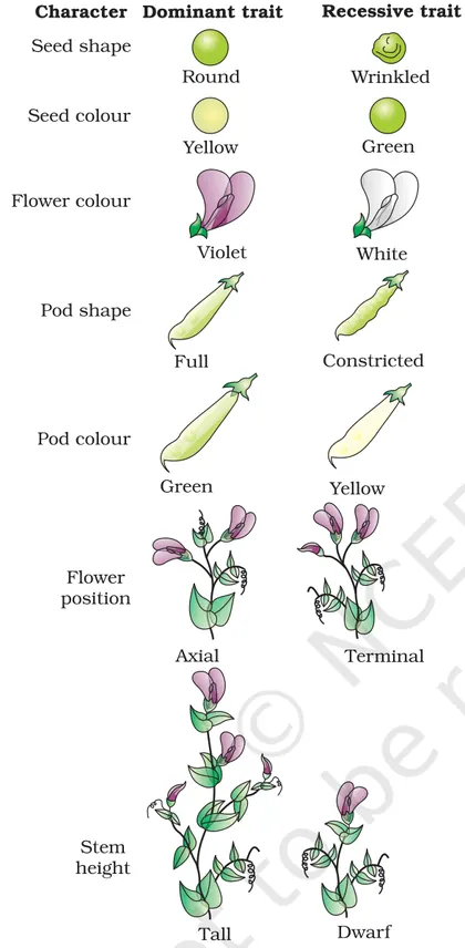
- Mendel's original pea traits: seed shape (round versus wrinkled), seed colour (yellow versus green), flower colour (purple versus white), pod shape, pod colour, flower position, stem length.
- Human autosomal dominant trait example: Huntington's disease (dominant allele causes disease).
- Human autosomal recessive example: Cystic fibrosis (disease appears when individual is homozygous recessive).
- ABO blood group: example of multiple alleles and codominance (IA and IB are codominant; IO is recessive).
- Sickle cell trait: demonstrates codominance/heterozygote advantage — heterozygotes (AS) have some resistance to malaria while homozygotes (SS) have disease.
- Monohybrid F2 phenotypic ratio (dominant : recessive) = 3 : 1
- Monohybrid F2 genotypic ratio (AA : Aa : aa) = 1 : 2 : 1
- Dihybrid F2 phenotypic ratio = 9 : 3 : 3 : 1 (both dominant : dominant-recessive : recessive-dominant : both recessive)
- Test cross predictions: If unknown is homozygous dominant (AA) x aa -> 100% dominant phenotype; if heterozygous (Aa) x aa -> 50% dominant : 50% recessive
- Probability (independent events) = product of individual probabilities (e.g., P(R and Y) = P(R) * P(Y))
- Chi-square (goodness of fit): Χ2 = Σ (observed - expected)^2 / expected ; degrees of freedom = (number of categories - 1)
Mendel's laws
Introduction: Mendel's laws are the foundational principles of classical genetics, formulated by Gregor Johann Mendel in the mid‑19th century from his hybridization experiments on Pisum sativum (garden pea). Mendel proposed simple rules that explain how traits are inherited from one generation to the next.
Key terms: gene (unit of heredity), allele (alternate form of a gene), genotype (genetic constitution), phenotype (observable trait), homozygous (two identical alleles, e.g., TT or tt), heterozygous (two different alleles, e.g., Tt), dominant (allele expressed in heterozygote), recessive (allele masked in heterozygote), gametes (sex cells).
1. Law of Dominance
Statement: When two homozygous individuals with contrasting traits are crossed (e.g., TT × tt), the trait that appears in the F1 hybrids is called dominant and the trait that is masked is called recessive.
Explanation: In the F1 generation of a monohybrid cross between homozygous dominant and homozygous recessive parents, all offspring are phenotypically like the dominant parent because the dominant allele masks the effect of the recessive allele in a heterozygote.
2. Law (Principle) of Segregation
Statement: During formation of gametes, paired alleles segregate (separate) so that each gamete receives only one allele of each gene. After fertilization, the pair is restored.
Explanation: In a heterozygote (Tt), the two alleles segregate during meiosis into different gametes; therefore half the gametes carry T and half carry t. On selfing or crossing heterozygotes (Tt × Tt) the genotype ratio in F2 is 1 TT : 2 Tt : 1 tt and the phenotype ratio (with complete dominance) is 3 dominant : 1 recessive.
3. Law (Principle) of Independent Assortment
Statement: Alleles of different genes assort independently of one another during gamete formation, provided the genes are on different (non‑homologous) chromosomes or far apart on the same chromosome.
Explanation: In a dihybrid cross (e.g., RrYy × RrYy for seed shape R/r and color Y/y), the alleles for shape segregate independently of alleles for color so gametes form in combinations (RY, Ry, rY, ry) with equal frequency. The F2 phenotypic ratio is 9:3:3:1 for two independently assorting, completely dominant gene pairs.
Experimental basis
- Monohybrid cross: Mendel crossed true‑breeding tall (TT) with dwarf (tt) peas. F1 all tall (Tt). F2 after selfing F1 gave 3 tall : 1 dwarf.
- Dihybrid cross: Mendel crossed RRYY (round yellow) with rryy (wrinkled green). F1 all RrYy (round yellow). F2 showed phenotypic ratio 9 round yellow : 3 round green : 3 wrinkled yellow : 1 wrinkled green.
- Test cross: Crossing an individual of unknown genotype with a homozygous recessive helps determine its genotype. Example: T? × tt gives 1:1 ratio if T? = Tt, or all tall if T? = TT.
Limitations and exceptions
- Linked genes (close on same chromosome) do not assort independently unless crossing over occurs.
- Incomplete dominance and codominance: heterozygote shows intermediate phenotype (e.g., Mirabilis jalapa) or both alleles expressed (ABO blood group).
- Multiple alleles, pleiotropy, epistasis, polygenic inheritance and environmental effects can modify Mendelian ratios.
Applications: Predicting inheritance of traits, plant and animal breeding, genetic counseling (with caveats), understanding molecular genetics and population genetics.
Note: Mendel's laws apply strictly for single‑gene traits with complete dominance and for genes that assort independently; modern genetics extends these rules to include linkage, molecular mechanisms and quantitative inheritance.
- Monohybrid cross (pea plant height): TT (tall) × tt (dwarf) → F1 all Tt (tall). F1 selfed: Tt × Tt → F2 genotypes 1 TT : 2 Tt : 1 tt, phenotypes 3 tall : 1 dwarf.
- Dihybrid cross (pea seed shape and color): RRYY × rryy → F1 all RrYy. F1 selfed → F2 phenotypic ratio 9 round yellow : 3 round green : 3 wrinkled yellow : 1 wrinkled green (9:3:3:1).
- Test cross to determine genotype: Cross unknown tall plant (T?) with homozygous recessive tt. If offspring ratio is 1 tall : 1 dwarf → parent was Tt. If all offspring tall → parent was TT.
- Human example (dominant vs recessive): Huntington's disease is inherited as an autosomal dominant trait (one mutant allele sufficient). Cystic fibrosis is autosomal recessive (requires two mutant alleles).
- Non‑Mendelian example: ABO blood groups show multiple alleles and codominance: A and B are codominant; O is recessive.
- Incomplete dominance example: Red (RR) × white (rr) Mirabilis jalapa gives pink (Rr) F1—heterozygote shows intermediate phenotype.
- Monohybrid F2 genotype ratio: 1 : 2 : 1 (AA : Aa : aa)
- Monohybrid F2 phenotype ratio (complete dominance): 3 : 1 (dominant : recessive)
- Dihybrid F2 phenotype ratio (independent assortment): 9 : 3 : 3 : 1
- Test cross (monohybrid) expected ratio if unknown is heterozygote: 1 : 1 (dominant : recessive)
- Number of types of gametes produced by an individual = 2^n, where n = number of heterozygous gene pairs
- Number of different genotypes possible in F2 (for n independently assorting loci) = 3^n
Monohybrid and Dihybrid crosses
Overview
Monohybrid and dihybrid crosses are classical Mendelian genetic crosses used to study inheritance of one trait (monohybrid) or two traits (dihybrid). These crosses demonstrate Mendel's laws: law of dominance, law of segregation (for a single gene) and law of independent assortment (for two or more genes that assort independently).
Monohybrid cross (one gene, two alleles)
- Definition: A cross between two individuals that differ in a single trait (one gene) — e.g., R (round) vs r (wrinkled) seeds in pea.
- Genotypes and alleles: Each individual has two alleles (AA, Aa, or aa). If A is dominant over a, phenotype follows A when present.
- Punnett square: For a cross between two heterozygotes (Aa × Aa) use a 2×2 Punnett square. Gametes: A and a from each parent.
- Expected F2 results (Aa × Aa): Genotypic ratio = 1 AA : 2 Aa : 1 aa. Phenotypic ratio (complete dominance) = 3 dominant : 1 recessive.
- Test cross: Crossing an individual with unknown dominant phenotype (A_) with a homozygous recessive (aa) reveals genotype. If any recessive phenotype appears, the tested parent was heterozygous.
Dihybrid cross (two independent genes)
- Definition: A cross between individuals differing in two traits controlled by two genes — e.g., seed shape (R/r) and seed colour (Y/y) in pea plants.
- Independent assortment: If genes are on different chromosomes or assort independently, alleles of one gene segregate independently of alleles of the other gene.
- F1 from true-breeding parents (RRYY × rryy) is RrYy (all dihybrid). Crossing two F1 individuals (RrYy × RrYy) is a dihybrid cross; use a 4×4 Punnett square or forked-line method.
- Expected F2 phenotypic ratio (RrYy × RrYy) = 9 : 3 : 3 : 1 (9 both dominant : 3 dominant first recessive second : 3 recessive first dominant second : 1 both recessive).
How ratios derive (multiplication rule)
Because segregation of each gene is independent, the probability of combined outcomes is the product of single-gene probabilities. Example: probability of dominant phenotype for gene R in F2 = 3/4; for Y = 3/4. So probability of both dominant = (3/4) × (3/4) = 9/16, giving the 9 part of 9:3:3:1.
Exceptions and complications
Real situations may deviate from simple Mendelian ratios due to linkage (genes close on the same chromosome), epistasis (one gene masks another), incomplete dominance, codominance, multiple alleles, polygenic inheritance, or environmental effects.
Study tips
Always list parental genotypes, write gametes, draw Punnett squares (2×2 for monohybrid, 4×4 for dihybrid) or use forked-line method, and convert genotype counts to phenotypic ratios.
- Monohybrid: Pea seed shape — Round (R) is dominant to wrinkled (r). Cross RR × rr → F1 all Rr (round). F1 × F1 (Rr × Rr) → F2 phenotypic ratio 3 round : 1 wrinkled; genotypic ratio 1 RR : 2 Rr : 1 rr.
- Monohybrid test cross: Unknown round pea (could be RR or Rr) crossed with rr. If all offspring are round → parent was RR; if approx. half round and half wrinkled → parent was Rr.
- Dihybrid: Mendel’s seed shape and colour — RRYY (round yellow) × rryy (wrinkled green) → F1 all RrYy. F1 × F1 (RrYy × RrYy) → F2 phenotypic ratio 9 round yellow : 3 round green : 3 wrinkled yellow : 1 wrinkled green (assuming independent assortment).
- Non-Mendelian example (incomplete dominance): Snapdragon flower colour — Red (RR) × White (rr) → F1 pink (Rr). F1 × F1 gives 1 red : 2 pink : 1 white (genotypic = phenotypic here).
- Codominance example: Human ABO blood group — IA and IB are codominant; IAIB genotype gives AB phenotype (both antigens expressed).
- Monohybrid (heterozygote × heterozygote): Genotypic ratio = 1 : 2 : 1 (AA : Aa : aa); Phenotypic ratio (complete dominance) = 3 : 1.
- Dihybrid (double heterozygote × double heterozygote): Phenotypic ratio = 9 : 3 : 3 : 1 (for two independently assorting genes).
- Probability of combined independent events: P(A and B) = P(A) × P(B). Use to derive dihybrid ratios (e.g., (3/4)×(3/4)=9/16).
- Number of possible genotypes for n independent loci (each with 2 alleles, complete dominance) = 3^n (each locus: AA, Aa, aa).
- Number of phenotypes under complete dominance for n loci = 2^n.
- Number of gamete types produced by an individual heterozygous at n loci = 2^n; Punnett square size (rows × columns) for two such parents = 2^n × 2^n, total boxes = 4^n.
Test cross, back cross and experimental design
Overview
Test cross and back cross are classical genetic crossing methods used to determine unknown genotypes and to transfer desirable traits into a given genetic background. Experimental design in genetics refers to planning crosses and analyses so results are statistically valid and biologically meaningful.
Test cross
Definition: A test cross is a cross between an individual showing the dominant phenotype (but unknown genotype) and an individual homozygous recessive for the trait. Purpose: to reveal whether the unknown parent is homozygous dominant or heterozygous.
Procedure & interpretation (monohybrid):
- Cross unknown (A–) with aabb (recessive homozygote, e.g., tt).
- If all offspring show the dominant phenotype → unknown was homozygous dominant (AA).
- If offspring segregate approximately 1 dominant : 1 recessive → unknown was heterozygous (Aa).
Dihybrid test cross: Cross a double heterozygote (AaBb) with aabb. Expected phenotypic ratio among offspring = 1:1:1:1 for the four phenotype classes (AB : Ab : aB : ab) if genes assort independently.
Back cross
Definition: A back cross is a cross between a hybrid (F1) and one of its parents or a genotype genetically similar to one parent (commonly the recurrent parent). Purpose: to recover parental genotype (recurrent parent) while retaining one or a few desired traits from the donor.
Uses: introgression of desirable alleles (e.g., disease resistance) into an elite cultivar; genetic mapping; confirmation of allele effects.
Genetic expectation after repeated backcrossing: Repeated backcrosses increase the proportion of the recurrent parent genome in the progeny while maintaining the selected donor allele.
Experimental design (in genetics)
Good experimental design ensures reliable conclusions from crosses and segregation data. Key elements:
- Clear objective / hypothesis: e.g., determine whether an individual is heterozygous for tallness.
- Parental selection: choose true-breeding (homozygous) parents for clear expectations.
- Controls: use known genotypes/phenotypes as positive and negative controls.
- Replication: perform multiple independent crosses and grow sufficient progeny to reduce sampling error.
- Sample size: large enough to reveal expected Mendelian ratios (use power thinking; small samples can deviate by chance).
- Randomization and blinding: randomize planting/measurement order and, where possible, blind phenotype scoring to reduce bias.
- Data recording & classification: clearly define phenotype categories and record counts.
- Statistical analysis: e.g., chi-square goodness-of-fit to compare observed counts with expected Mendelian ratios.
- Repeat & confirm: repeat crosses or validate results using reciprocal crosses or molecular genotyping if available.
Statistical check — Chi-square test (goodness of fit)
Use chi-square (χ2) to test whether observed segregation differs significantly from expected ratios.
Formula: χ2 = Σ (O − E)² / E, where O = observed count, E = expected count. Degrees of freedom (d.f.) = (number of categories − 1). Compare χ2 to critical value at chosen significance level (usually 0.05).
Practical notes
- Environmental factors can affect phenotype expression; use controlled conditions where possible.
- Linked genes deviate from independent assortment; recombination frequency and mapping are required.
- Molecular markers and genotyping now often replace or complement phenotypic test crosses.
- Mendel's pea experiment (monohybrid test cross idea): To test whether a tall pea plant with dominant phenotype (T–) is TT or Tt, cross it with tt: if all F1 are tall → TT; if roughly 1:1 tall:short → Tt.
- Dihybrid test cross: Cross AaBb (round yellow) with aabb (wrinkled green). Expected offspring phenotypes (round yellow : round green : wrinkled yellow : wrinkled green) ≈ 1:1:1:1 if genes are unlinked.
- Crop breeding (backcrossing): Introgressing disease-resistance allele from a donor plant into an elite variety by crossing F1 to the elite parent repeatedly while selecting for resistance. After n backcrosses the recurrent parent genome fraction approaches 1 (see formula).
- Animal breeding: Backcrossing a hybrid mouse carrying a mutant allele to a wild-type parent strain to place the mutation on a standard genetic background for experiments.
- Monohybrid test cross expectation: Unknown (A–) × aa → offspring ratios: if AA × aa → all Aa (dominant phenotype). If Aa × aa → 1 Aa : 1 aa (dominant : recessive).
- Dihybrid test cross expectation: AaBb × aabb → phenotypic ratio ≈ 1 : 1 : 1 : 1 for the four phenotype classes (assuming independent assortment).
- Backcross recurrent-parent genome after n backcrosses: Proportion = 1 − (1/2)^(n+1). Example: after 1 backcross = 1 − (1/2)^2 = 3/4 = 75%; after 2 = 87.5%.
- Chi-square test: χ² = Σ (O − E)² / E ; degrees of freedom = (number of categories − 1). Compare χ² to critical value at chosen α (commonly 0.05).
Statistical analysis in genetics
What it is: Statistical analysis in genetics is the use of probability and statistical tests to decide whether observed genetic data (phenotypes or genotypes) fit expected patterns based on Mendelian inheritance or other genetic models. It helps distinguish between differences due to chance and those due to a real biological cause.
Core ideas:
- Probability rules (addition and multiplication) are used to predict expected ratios of offspring (e.g., 3:1 for a monohybrid cross, 9:3:3:1 for a dihybrid cross).
- The Chi-square (χ²) test (goodness-of-fit) is used to compare observed counts with expected counts and evaluate whether deviations are due to chance.
- Null hypothesis (H0): observed deviations from expected ratios are due to random sampling (chance). If χ² is small enough (below critical value), we accept H0; if large, we reject H0.
Chi-square test — steps:
- State H0 and choose significance level (usually α = 0.05).
- Calculate expected numbers for each category: E = (expected proportion) × (total observed).
- Compute χ² = Σ (O − E)² / E, summing over all categories.
- Degrees of freedom (df) = number of categories − 1.
- Compare calculated χ² with critical χ² value from chi-square table at chosen α and df. If χ² ≤ χ²_critical, accept H0 (differences are by chance); if χ² > χ²_critical, reject H0.
Worked example (monohybrid, expected 3:1):
Suppose a cross gives 65 dominant phenotype and 35 recessive phenotype (total 100). Expected ratio 3:1 → expected numbers = 75 dominant, 25 recessive.
Compute χ²: χ² = (65−75)²/75 + (35−25)²/25 = 100/75 + 100/25 = 1.333 + 4 = 5.333.
df = 2 − 1 = 1. For α = 0.05, χ²_critical(1) = 3.84. Since 5.333 > 3.84, reject H0 → deviation is unlikely due to chance alone.
Other statistical tools in genetics: probability calculations for gamete combinations (using multiplication rule), binomial expansion for multi-event probabilities, and descriptive statistics (mean, variance, standard deviation) for quantitative traits.
Interpretation caveats: A significant χ² does not specify the cause of deviation — possible reasons include linkage, selection, small sample size, experimental error or misclassification, non-Mendelian inheritance, or environmental effects. Always consider biological context.
Practical uses / applications: testing Mendel's ratios in crosses, checking whether a sample fits Hardy–Weinberg expectations (population genetics), validating expected segregation of markers in breeding experiments, and assessing association between genotype and phenotype.
- Monohybrid cross (pea seeds): Observed 65 yellow : 35 green (total 100). Expected 3:1 → 75 : 25. χ² = 5.333, df = 1 → χ² > 3.84 → reject null (deviation unlikely by chance).
- Dihybrid cross (seed shape & color): Expected phenotypic ratio 9:3:3:1. If observed counts differ, calculate expected counts by multiplying total by each proportion (e.g., expected for 9/16 = total×9/16) and perform χ² test with df = 4−1 = 3.
- Blood group proportions in a sample: Suppose you expect population proportions (A:B:AB:O). Use χ² to test if a sample's observed counts match expected population frequencies.
- Probability example: If two heterozygotes (Aa × Aa) mate, probability of aa offspring = P(a from parent1) × P(a from parent2) = (1/2) × (1/2) = 1/4.
- Chi-square: χ² = Σ (O − E)² / E (sum over all phenotype/genotype categories)
- Expected count: E = (expected proportion) × (total observed)
- Degrees of freedom: df = (number of categories) − 1
- Addition rule (exclusive events): P(A or B) = P(A) + P(B); General: P(A or B) = P(A) + P(B) − P(A and B)
- Multiplication rule (independent events): P(A and B) = P(A) × P(B)
- Mean (sample): x̄ = (Σ xi) / n
Deviations from Mendelian inheritance
Introduction: Mendel's laws (law of segregation and independent assortment) describe simple dominant–recessive inheritance for single-gene traits. Many real traits however do not follow these simple Mendelian ratios. These departures arise when alleles interact, more than two alleles exist, genes are linked, inheritance is influenced by sex or cytoplasm, or when alleles affect viability.
Main types of deviations:
- Incomplete dominance — heterozygote shows intermediate phenotype. Example: snapdragon flower colour (red × white → pink). F2 phenotypic ratio = 1 red : 2 pink : 1 white.
- Co-dominance — both alleles expressed equally in heterozygote. Example: ABO blood group (IA and IB co‑dominant; i is recessive). Genotypic ratio 1:2:1 may correspond to three or four phenotypes depending on alleles.
- Multiple alleles — more than two allelic forms in a population (e.g., ABO: IA, IB, i). Organism still diploid but multiple possible genotypes/phenotypes exist.
- Pleiotropy — a single gene affects multiple, seemingly unrelated traits. Example: phenylketonuria (PKU) causes metabolic defect and neurological effects; sickle‑cell allele affects RBC shape, resistance to malaria, and vaso‑occlusive symptoms.
- Polygenic inheritance (quantitative traits) — many genes contribute additively to a trait (continuous distribution). Examples: human height, skin colour. Phenotype shows a bell‑shaped distribution; environment also influences expression.
- Gene interaction (epistasis) — alleles at one locus mask or modify expression at another locus. Typical ratios in a dihybrid F2 differ from 9:3:3:1. Common patterns:
- Recessive epistasis: 9:3:4 (example: coat colour in mice/labrador retriever where ee masks B/b)
- Dominant epistasis I: 12:3:1 (example: some squash fruit colours)
- Complementary (both genes required): 9:7 (example: flower colour in sweet pea)
- Duplicate genes (either gene sufficient): 15:1
- Sex‑linked inheritance — genes on sex chromosomes show patterns different from autosomes. Example: X‑linked recessive traits such as haemophilia and red–green colour blindness; males more frequently affected.
- Sex‑influenced and sex‑limited traits — expression depends on sex hormones/background. Example: male pattern baldness (sex‑influenced), milk production (sex‑limited to females; trait controlled by autosomes but expressed only in one sex).
- Linkage and crossing over — genes located close together on same chromosome do not assort independently; parental (nonrecombinant) types are more frequent than recombinants. Recombination frequency is used to map gene distance.
- Cytoplasmic (maternal) inheritance — genes present in organelles (mitochondria, chloroplasts) are transmitted almost exclusively from the mother. Example: mitochondrial disorders (Leber's hereditary optic neuropathy); variegation in Mirabilis jalapa (4 o'clock plant).
- Lethal alleles — certain genotypes cause death (often embryonic), altering observed ratios. Example: yellow coat A^Y allele in mice is dominant for colour but homozygous A^Y/A^Y is lethal, producing altered F2 ratios.
Molecular & population basis: Non‑Mendelian outcomes arise because genes can interact in metabolic pathways, multiple alleleic forms exist, chromosomal arrangement (linkage) restricts independent assortment, organellar genomes follow uniparental inheritance, and selection or viability differences distort expected counts.
How geneticists detect deviations:
- Use test crosses and F1/F2 ratios (Punnett squares) and compare observed vs expected counts.
- Chi‑square (χ2) goodness‑of‑fit test to assess whether deviation is statistically significant.
- Measure recombination frequencies to detect linkage and construct genetic maps (centimorgans).
Importance: Recognising deviations is essential for predicting inheritance of complex traits, genetic counseling (e.g., sex‑linked disorders), breeding programs, and understanding population genetics and evolution.
Summary: Mendel laid the foundation, but many biologically important traits follow patterns that depart from simple Mendelian ratios due to dominance relationships, multiple alleles, gene interactions, linkage, sex or cytoplasmic effects, pleiotropy, lethality and polygenic inheritance.
- Incomplete dominance: Snapdragon (Antirrhinum) — red × white → pink in F1; F2 ratio 1 red : 2 pink : 1 white.
- Co‑dominance and multiple alleles: Human ABO blood group — IA and IB co‑dominant; i recessive.
- Epistasis (recessive epistasis): Labrador retriever coat colour — B (black) vs b (brown) with E locus required for pigment; genotypic interactions give 9:3:4 phenotypic ratio.
- Complementary genes: Sweet pea flower colour — two genes both required for purple pigment, F2 ratio 9 purple : 7 white.
- Polygenic inheritance: Human height or skin colour — many genes additively affect phenotype producing continuous variation.
- Sex‑linked trait: Red–green colour blindness and haemophilia — X‑linked recessive conditions more common in males.
- Recombination frequency (RF) = (Number of recombinant offspring / Total offspring) × 100%; map distance ≈ RF in centimorgans (cM).
- Chi‑square (goodness of fit): χ² = Σ (observed − expected)² / expected. Compare to χ² table with appropriate degrees of freedom to test hypothesis.
- Hardy‑Weinberg (population allele/genotype frequencies) useful as baseline: p + q = 1; p² + 2pq + q² = 1 (for two alleles).
- Common expected phenotypic ratios for deviations: - Incomplete dominance/co‑dominance (monohybrid F2): 1 : 2 : 1 - Complementary genes (dihybrid F2): 9 : 7 - Duplicate genes: 15 : 1 - Recessive epistasis: 9 : 3 : 4 - Dominant epistasis I: 12 : 3 : 1
Incomplete dominance and codominance
Definition — Incomplete dominance: A form of non-Mendelian inheritance in which the heterozygote shows a phenotype intermediate between the two homozygotes (neither allele is completely dominant). Example genotype notation: RR (red) × rr (white) → Rr (pink).
Definition — Codominance: A pattern of inheritance in which both alleles in a heterozygote are fully and simultaneously expressed, producing a phenotype that clearly shows both parental traits (not blended).
Genetic basis: Incomplete dominance usually results from dosage effects or reduced activity of an allele product (haploinsufficiency): the heterozygote produces less pigment or product than the homozygous dominant, giving an intermediate appearance. Codominance arises when both allele products are produced and functional in the heterozygote, so both phenotypes appear independently.
F2 patterns: For a single gene with two alleles showing either incomplete dominance or codominance, a cross between two heterozygotes (Aa × Aa) gives genotypic ratio 1:2:1 (AA : Aa : aa) and a corresponding phenotypic ratio 1:2:1 because the heterozygote phenotype is distinct from either homozygote.
Key distinctions (quick):
- Incomplete dominance = intermediate/blended phenotype (e.g., red × white → pink).
- Codominance = both parental phenotypes visible together (e.g., red + white hairs = roan).
- Both deviate from classical dominant–recessive where heterozygote equals one homozygote.
Biological and clinical relevance: Many human blood group phenotypes and some molecular traits show codominance (both antigens or protein variants present). Some enzyme/pigment gene interactions show incomplete dominance because one functional allele does not give full wild-type output.
- Incomplete dominance — Snapdragon (Antirrhinum majus): Red (RR) × White (rr) → Pink (Rr) in F1; F2 phenotypic ratio = 1 red : 2 pink : 1 white.
- Incomplete dominance — Four o'clock (Mirabilis jalapa): red × white often gives pink (intermediate) flowers (classical textbook example).
- Codominance — Human ABO blood group: IA and IB are codominant; IAIB genotype expresses both A and B antigens → AB phenotype.
- Codominance — MN blood group: alleles L^M and L^N produce distinct glycoprotein forms; heterozygote shows both forms on RBCs.
- Codominance — Roan cattle: crossing red and white gives roan offspring with both red and white hairs mixed (both pigments expressed).
- Molecular example — Sickle-cell (HbA and HbS): at the protein level heterozygotes produce both normal and abnormal hemoglobin (often cited as codominant at molecular level), though clinical phenotype can be intermediate/variable.
- For monohybrid cross with two alleles (A and a) showing incomplete dominance or codominance: Aa × Aa → Genotype ratio = 1 AA : 2 Aa : 1 aa
- Corresponding phenotypic ratio = 1 (homozygote 1) : 2 (heterozygote distinct) : 1 (homozygote 2)
- Probability formulas (example): P(AA) = 1/4, P(Aa) = 1/2, P(aa) = 1/4 for Aa × Aa
- General notation: If allele A produces quantity x of product and allele a produces 0, incomplete dominance may result when Aa produces x/2 (intermediate). In codominance, Aa produces both products: amount_A > 0 and amount_a > 0 and both are detectable.
Multiple allelism
Definition: Multiple allelism (multiple alleles) occurs when a single gene locus has more than two alternative alleles present in a population. An individual diploid organism still carries only two alleles (one per homologous chromosome), but the population may have many different allelic forms.
Key points:
- Multiple alleles increase the number of possible genotypes and phenotypes in a population compared with simple two-allele systems.
- Different alleles may show simple dominance, recessiveness, co-dominance, incomplete dominance or an allele series (hierarchy of dominance).
- Multiple allelism is distinct from polygenic inheritance (many genes affecting one trait) and from pleiotropy (one gene affecting many traits).
Classical example — ABO blood group system (humans):
The ABO locus has three common alleles: IA, IB and i. IA and IB are co-dominant to each other and each is dominant over i. Possible genotypes and phenotypes:
- IAIA or IAi → Blood group A
- IBIB or IBi → Blood group B
- IAIB → Blood group AB (co-dominance)
- ii → Blood group O
Pedigree and crosses: Use a 3×3 Punnett square for crosses between two heterozygotes carrying different alleles (e.g., IAi × IBi gives 1 IAIB : 1 IAi : 1 IBi : 1 ii → A : B : AB : O = 1:1:1:1).
Special cases related to multiple allelism:
- Bombay (hh) phenotype: A rare mutation at the H locus prevents formation of the H antigen (precursor). Individuals with genotype hh can appear as group O regardless of ABO genotype because the A and B antigens cannot be attached. This demonstrates interaction between loci (epistasis) combined with multiple alleles at ABO.
- Allelic series: Example — C locus in rabbits (alleles C > cch > ch > ca > c) where there is a dominance hierarchy among several alleles determining coat color.
Population genetics with multiple alleles:
For n alleles with frequencies p1, p2, …, pn (sum = 1), the expected genotype frequencies under Hardy–Weinberg equilibrium are:
- Homozygotes: pi2 for each allele i
- Heterozygotes: 2 pi pj for each distinct pair i ≠ j
These relationships allow calculation of phenotype frequencies for systems like ABO by summing the relevant genotype frequencies (e.g., frequency of A = pA2 + 2 pA pO if pA, pB, pO denote allele frequencies for IA, IB, i respectively).
Distinguishing points students should remember:
- Multiple alleles: >2 alleles in population; individual is diploid (max two alleles per individual).
- Co-dominance example: IA and IB show both phenotypes in AB individuals.
- Dominance hierarchy (allelic series) is common in traits such as coat color.
- ABO blood group system (I^A, I^B, i): co-dominance of I^A and I^B; both are dominant over i.
- Bombay (hh) phenotype: interaction of H locus with ABO alleles producing apparent O phenotype despite A/B alleles.
- Rabbit C-locus allelic series (C > cch > ch > ca > c) determining coat color variants.
- HLA (human leukocyte antigen) genes: extremely polymorphic with many alleles (important in transplantation).
- For n alleles with frequencies p1, p2, ..., pn: sum(p_i) = 1
- Genotype frequencies (Hardy–Weinberg, multiple alleles): homozygote for allele i = p_i^2; heterozygote for alleles i and j = 2 p_i p_j (i ≠ j)
- For three alleles p,q,r: p + q + r = 1 and genotype terms: p^2 + q^2 + r^2 + 2pq + 2pr + 2qr = 1
- Example (ABO): frequency(A) = p^2 + 2pr, frequency(B) = q^2 + 2qr, frequency(AB) = 2pq, frequency(O) = r^2 (where p = freq(I^A), q = freq(I^B), r = freq(i))
Polygenic inheritance and quantitative traits
Definition: Polygenic inheritance (also called quantitative inheritance) is the control of a single phenotypic character by two or more genes (polygenes), each of which has a small additive effect. These traits show continuous variation in a population (a range of phenotypes rather than discrete categories).
Key features:
- Multiple genes (often unlinked) contribute additively to the phenotype.
- Each gene usually has two or more alleles; individual allele effects are small and cumulative.
- Traits show continuous variation (a smooth range of values) rather than discrete classes.
- Environmental factors influence the phenotype, so phenotype = genotype + environment (G + E).
- F2 and later-generation distributions tend to approximate a normal (bell-shaped) curve when many genes are involved.
Classical example and genetics: The Nilsson-Ehle wheat kernel colour experiment illustrated polygenic inheritance. When two homozygous lines differing in several contributing genes were crossed and F2 analysed, the offspring showed many intermediate colour classes (not simple Mendelian ratios). If n independent loci contribute additively, the number of phenotypic classes expected is 2n + 1.
Role of environment: Environmental variation (nutrition, temperature, etc.) modifies the phenotypic expression of polygenic traits and increases the continuous spread of values.
Variance components and heritability: For quantitative traits we partition phenotypic variance (Vp) into genetic and environmental parts. Important components and parameters used in quantitative genetics include:
- Vp = Vg + Ve (phenotypic variance = genetic variance + environmental variance) — simple partition.
- Vg can be subdivided into additive genetic variance (Va), dominance variance (Vd) and interaction/epistatic variance (Vi): Vg = Va + Vd + Vi.
- Broad-sense heritability H2 = Vg / Vp (fraction of phenotypic variance due to all genetic factors).
- Narrow-sense heritability h2 = Va / Vp (fraction due to additive genetic variance) — important for predicting response to selection.
Selection and response: The expected response to artificial selection is given by R = h2 × S, where S is the selection differential (difference between mean of selected parents and mean of original population). This shows why additive variance (Va) is crucial for breeding.
Why a bell curve? When many independent genes each contribute small effects, the combined distribution of phenotypes follows the central limit theorem and approximates a normal (Gaussian) distribution. This explains the continuous, smooth frequency distribution seen for traits like height or weight.
Practical importance: Understanding polygenic inheritance is essential in plant and animal breeding, human genetics (e.g., risk for complex diseases), and evolutionary studies of continuous traits.
- Human height (classic polygenic trait influenced by many genes and environment).
- Human skin colour (multiple pigment-producing genes; continuous variation).
- Body weight and BMI (genetic and environmental contributions).
- Grain yield and size in crop plants (controlled by many genes; breeding targets).
- Milk yield in cattle (quantitative trait used in selective breeding).
- Fur colour intensity in some animals where several loci additively affect pigment.
- Number of phenotypic classes = 2n + 1 (n = number of independent polygenes).
- Vp = Vg + Ve (phenotypic variance = genetic variance + environmental variance).
- Vg = Va + Vd + Vi (genetic variance = additive + dominance + interaction/epistatic variance).
- Broad-sense heritability: H^2 = Vg / Vp.
- Narrow-sense heritability: h^2 = Va / Vp.
- Response to selection: R = h^2 × S, where S = mean(selected parents) - mean(population).
Pleiotropy and gene interactions
Pleiotropy
Definition: Pleiotropy occurs when a single gene influences two or more seemingly unrelated phenotypic traits. A mutation in that gene therefore produces multiple effects in the organism.
Mechanisms:
- Single gene product has multiple functions in different tissues (e.g., structural protein used in many organs).
- Gene acts in a developmental cascade — a change early in development affects many downstream traits.
- One gene product influences a biochemical pathway affecting several traits (metabolic pleiotropy).
Consequences: Pleiotropic genes make prediction of phenotype from genotype more complex because one mutation can cause a syndrome of traits; important in human genetic disease and evolutionary constraints.
Gene interactions (epistasis and related types)
Definition: Gene interaction refers to the phenomenon where alleles of two or more different genes influence the same trait and the combined effect on phenotype is non-additive (the phenotype is not simply the sum of individual gene effects). Epistasis is a form of gene interaction where one gene masks or modifies the expression of another gene.
Basic idea using dihybrid crosses: For two independently assorting genes (AaBb × AaBb) the genotypic ratio in F2 is 9:3:3:1. Different types of interactions change how those 16 genotypic classes are grouped into phenotypes, producing characteristic phenotypic ratios.
Common types of gene interactions (with typical F2 phenotypic ratios):
- Complementary (both genes required): 9 : 7 — two genes produce a trait only when both have at least one dominant allele (A-B-). Example: flower pigmentation pathways where two enzymes are required.
- Duplicate (redundant genes): 15 : 1 — either dominant allele of two genes gives the same phenotype (either A- or B- produces trait).
- Recessive epistasis: 9 : 3 : 4 — homozygous recessive at one locus (ee) masks expression of B/b (seen in Labrador coat colour; E controls pigment deposition; ee → yellow regardless of B).
- Dominant epistasis (type I): 12 : 3 : 1 — a dominant allele at one locus masks the expression of alleles at the second locus (examples: some squash fruit colour patterns).
- Dominant suppression / inhibitory epistasis: 13 : 3 — one dominant allele suppresses expression of the other gene except in the double recessive class.
Molecular/biochemical perspective: Gene interactions often reflect steps in biochemical pathways. If enzyme A (product of gene A) acts upstream of enzyme B (gene B), a loss of A can prevent the substrate reaching B — making A epistatic to B. Epistasis therefore reveals pathway order.
Distinction from polygenic inheritance: Gene interaction refers to interplay between a few genes controlling a single trait qualitatively (discrete classes). Polygenic (quantitative) inheritance involves many genes each contributing additively to continuous variation (height, weight).
Summary points
- Pleiotropy: one gene, many traits. No single numeric "ratio"—effects are descriptive or clinical.
- Gene interactions: phenotype depends on combinations of alleles at different loci; classical ratios (9:7, 15:1, 9:3:4, 12:3:1, 13:3) help identify interaction type.
- Epistasis can be used to infer biochemical pathway order and regulatory relationships.
- Pleiotropy — Phenylketonuria (PKU): mutation in PAH gene (phenylalanine hydroxylase) leads to high phenylalanine and causes intellectual disability, hypopigmentation and musty odour — multiple symptoms from one gene defect.
- Pleiotropy — Sickle cell disease: a single amino-acid substitution in HBB causes sickled red cells (anaemia), vaso-occlusive crises, and confers malaria resistance (multiple effects of one mutation).
- Pleiotropy — Marfan syndrome: mutation in FBN1 affects connective tissue resulting in long limbs, lens dislocation and aortic aneurysm.
- Recessive epistasis — Labrador retriever coat colour: B (black) vs b (brown) determines pigment; E (pigment deposition) vs e (no deposition). Genotypes with ee are yellow regardless of B/b, giving a 9:3:4 phenotypic ratio (black:brown:yellow).
- Complementary genes — Flower colour in some plants: two different enzymes required to synthesise pigment; only A-B- produce coloured flowers while other combinations produce white (9:7).
- Bombay phenotype (epistasis) — H gene required to produce H antigen for ABO blood groups; individuals with hh show O-like phenotype regardless of ABO genotype because antigen is not produced.
- Dihybrid F2 genotype proportions from AaBb × AaBb: 9:3:3:1 (derived from (3/4 × 3/4) : (3/4 × 1/4) : (1/4 × 3/4) : (1/4 × 1/4)).
- Probability principle for independent genes: P(genotype for A and genotype for B) = P(genotype for A) × P(genotype for B). Use product rule to compute expected classes.
- Common phenotypic ratios for two-gene interactions (F2 classes): Complementary 9:7; Duplicate 15:1; Recessive epistasis 9:3:4; Dominant epistasis 12:3:1; Dominant suppression 13:3.
- To test fit to an expected ratio: X² = Σ((observed − expected)² / expected) where expected = total × (expected fraction for each class).
Chromosomal basis of inheritance
Overview
The chromosomal basis of inheritance is the concept that genes are located on chromosomes and that the behaviour of chromosomes during meiosis and fertilisation explains inheritance patterns. This idea unifies Mendel’s laws with cytology and genetics.
Key historical points
- Sutton–Boveri hypothesis (early 1900s): chromosomes are the carriers of Mendelian factors (genes); paired chromosomes segregate during meiosis explaining segregation of alleles.
- Thomas Hunt Morgan (Drosophila): demonstrated that specific genes are located on specific chromosomes, discovered sex-linked inheritance and genetic linkage.
How chromosomes explain Mendel’s laws
- Segregation: during meiosis I homologous chromosomes (each carrying an allele of a gene) separate into different gametes — explains 1:1 segregation of alleles.
- Independent assortment: non-homologous chromosome pairs orient independently at metaphase I, explaining independent assortment of genes located on different chromosomes.
Linkage and recombination
Genes located close together on the same chromosome are said to be linked and tend to be inherited together (do not show independent assortment). Crossing over between homologous chromosomes during prophase I can exchange segments and produce recombinant chromosomes, creating new allele combinations. The frequency of recombination between two genes is proportional to the physical distance between them, enabling genetic mapping.
Genetic mapping
Recombination frequency (measured in percentage) is used to estimate map distances in centiMorgans (cM): 1% recombination ≈ 1 cM. With three-point crosses and recombination data, gene order and distances can be determined.
Sex chromosomes and sex-linked inheritance
Sex chromosomes (e.g., X and Y in humans, Z and W in birds) carry genes that show sex-linked inheritance. X-linked recessive traits (e.g., haemophilia, red-green colour blindness) more often affect males because males are hemizygous for X. Y chromosome carries male-specific genes (e.g., SRY) important for sex determination.
Dosage compensation (X-inactivation)
In mammals, one X chromosome in females is randomly inactivated (Lyon hypothesis) so that X-linked gene expression between XX females and XY males is balanced. Inactivated X forms a Barr body.
Chromosomal aberrations and disorders
Structural and numerical chromosomal changes affect inheritance and phenotype. Types include:
- Numerical: aneuploidy (trisomy 21 — Down syndrome; 45,X — Turner; 47,XXY — Klinefelter).
- Structural: deletions, duplications, inversions, translocations (e.g., Robertsonian translocation between 14 and 21 can cause familial Down syndrome).
Evidence from experiments and observations
- Cytological correlation: specific mutations map to specific chromosomes (staining, banding, karyotyping).
- Mutant phenotypes in model organisms (Drosophila): eye colour, wing mutations mapped to X chromosome led to discovery of sex-linked inheritance.
- Linkage maps constructed from recombination data correlate with physical chromosome maps.
Applications
Diagnosis of chromosomal disorders (karyotyping, FISH), prenatal testing, genetic counselling, constructing linkage maps for breeding and gene mapping in research.
Summary
The chromosomal basis of inheritance places genes on chromosomes and uses chromosome behaviour during meiosis to explain Mendelian segregation, linkage, recombination and patterns of inheritance including sex-linked traits and chromosomal disorders.
- Thomas Hunt Morgan’s Drosophila experiments: discovery that the gene for white eye is on the X chromosome (X‑linked) and demonstrates sex-linked inheritance.
- Haemophilia in humans: X‑linked recessive disorder — mostly affects males who inherit the mutated allele from carrier mothers.
- Red–green colour blindness: X‑linked recessive trait; females must have two mutant X alleles to be colour-blind, males need only one.
- Down syndrome (trisomy 21): numerical chromosomal aberration causing characteristic phenotype and intellectual disability.
- Robertsonian translocation (14;21): a parent with a balanced translocation can produce offspring with unbalanced karyotype resulting in familial Down syndrome.
- Recombination frequency (%) = (Number of recombinant offspring / Total offspring) × 100
- Map distance (in centiMorgans, cM) ≈ Recombination frequency (%)
- Chi-square (goodness of fit) = Σ[(Observed − Expected)² / Expected] (used to test genetic ratios)
- Coefficient of coincidence (c.c.) = Observed double crossovers / Expected double crossovers
- Interference (I) = 1 − Coefficient of coincidence
Linkage and crossing over
Introduction
Linkage is the tendency of genes that are located close together on the same chromosome to be inherited together. Genes on different (non-homologous) chromosomes or far apart on the same chromosome usually follow Mendel's law of independent assortment; linked genes do not, unless crossing over separates them.
Mechanism — Crossing over
Crossing over (genetic recombination) occurs during prophase I of meiosis when homologous chromosomes pair (synapsis) and exchange corresponding segments at points called chiasmata. Crossing over produces recombinant chromosomes that carry new combinations of alleles, breaking linkage between genes.
Types of linkage
- Complete linkage: Genes are so close that no crossing over occurs between them in the observed sample — only parental (nonrecombinant) types appear.
- Incomplete (partial) linkage: Crossing over occurs occasionally between the genes — both parental and recombinant offspring are produced. The proportion of recombinants reflects the physical distance between the genes.
Linkage phase
For a pair of heterozygous loci, parental allele configurations may be in coupling (cis) — both dominant alleles on one homolog and both recessive on the other — or repulsion (trans) — dominant and recessive alleles are mixed on each homolog. The phase affects which phenotypes are parental vs recombinant but not recombination frequency.
Detecting linkage — test cross
A common experimental design is to cross a dihybrid (AaBb) with a double homozygous recessive (aabb). If genes assort independently, four phenotypic classes occur in equal frequencies. If linked, parental types are more frequent than recombinants; recombination frequency (RF) is calculated from offspring counts and used to estimate map distance.
Gene mapping
Recombination frequency is proportional (approximately) to physical distance for short distances. Map distance is expressed in map units or centimorgans (cM): 1% recombination = 1 cM. For three genes, use three-point test crosses to determine gene order and distances; double crossover classes (least frequent) reveal the gene order.
Limits and special topics
- Maximum observed recombination frequency between two loci is 50% — beyond that they behave as if unlinked.
- Coefficient of coincidence (c.o.c.) measures how many double crossovers actually occur compared with expected. Interference = 1 − c.o.c. Positive interference means fewer double crossovers than expected.
Biological significance
Crossing over increases genetic variation in gametes, providing raw material for evolution. Linkage information is used in genetic mapping, pedigree analysis, and marker-assisted breeding.
- Thomas Hunt Morgan's Drosophila experiments: Morgan observed that certain pairs of traits (e.g., body color and wing shape) were inherited together more often than expected by independent assortment; occasional recombinant flies showed crossing over between the linked genes.
- Human X-linked traits: Hemophilia and red–green color blindness are both X‑linked. In pedigree analysis these traits often appear together in males, illustrating physical linkage on the X chromosome (crossing over in female meiosis can separate them occasionally).
- Plant and animal breeding: Marker-assisted selection uses linkage between a visible or molecular marker and a desirable gene (e.g., disease resistance) to select offspring more efficiently; recombination frequency determines how reliable the marker is.
- Three-point test cross example (practical exercise): A breeder crosses an individual heterozygous for three linked loci to a triple recessive tester to determine gene order and map distances — parental types are most frequent, single crossovers intermediate, double crossovers least frequent.
- Recombination frequency (RF) = (Number of recombinant offspring / Total number of offspring) × 100%
- Map distance (in centimorgans, cM) ≈ RF% (1% RF ≈ 1 cM) for small distances
- Expected frequency of double crossovers ≈ (RF between gene A & B) × (RF between gene B & C) [use proportions, not %]
- Coefficient of coincidence (c.o.c.) = (Observed number of double crossovers) / (Expected number of double crossovers)
- Interference (I) = 1 − c.o.c. (ranges from −∞ to 1; typically 0 ≤ I ≤ 1 in biological data)
Sex determination mechanisms
Overview
Sex determination mechanisms are biological processes that establish whether an embryo develops as male, female or intersex. Mechanisms may be chromosomal, genic, haplodiploid or environmental and differ among taxa. The developmental outcome often depends on a primary signal (chromosome constitution, gene product, temperature) that triggers a hormonal and gene-regulatory cascade producing gonads and secondary sexual characters.
1. Chromosomal sex determination
- XX/XY system (male heterogamety) — found in humans and many mammals. Females: XX, Males: XY. The presence of the Y chromosome (SRY gene) initiates testis formation. Typical cross: XX (mother) × XY (father) → 50% XX daughters, 50% XY sons.
- ZZ/ZW system (female heterogamety) — birds, butterflies. Males: ZZ (homogametic), Females: ZW (heterogametic). Here the female determines the sex of the offspring.
- XO system — grasshoppers, some insects. Females: XX, Males: XO (one X, no second sex chromosome). Sex determined by presence/absence of second sex chromosome.
- Multiple sex chromosomes — some species (e.g., platypus) have chains of X and Y chromosomes; combinations determine sex.
2. X:A ratio (Drosophila special case)
In Drosophila, sex is determined by the ratio of number of X chromosomes (X) to number of haploid sets of autosomes (A). X:A = 1.0 → female; X:A = 0.5 → male; intermediate ratios produce intersex or metafemale/metamale phenotypes.
3. Haplodiploidy
Found in Hymenoptera (bees, ants, wasps). Females are diploid (from fertilized eggs) and males are haploid (from unfertilized eggs). The queen can control sex by fertilizing or not fertilizing eggs.
4. Environmental sex determination (ESD)
Sex determined by external factors rather than chromosomes. Classic example: temperature-dependent sex determination (TSD) in many reptiles (turtles, some crocodiles). Incubation temperature during a critical embryonic period biases development toward male or female.
5. Genic sex determination and sex-determining genes
Some organisms lack distinct sex chromosomes; sex is determined by specific alleles at one or more loci. Key gene example in mammals: SRY on the Y chromosome encodes testis-determining factor (a transcription factor) that activates male pathway (SOX9, AMH) and suppresses female pathway. Mutations/translocations can produce sex-reversal (e.g., XX male if SRY translocated to X; XY female if SRY mutated or downstream pathway disrupted).
6. Consequences for inheritance
Chromosomal sex determination creates sex-linked inheritance patterns. For example, X-linked recessive disorders (e.g., hemophilia, color blindness) disproportionately affect males because males have only one X.
7. Human clinical examples
Aneuploidies involving sex chromosomes produce syndromes: Turner syndrome (45,X) — phenotypically female, short stature, ovarian failure; Klinefelter syndrome (47,XXY) — phenotypically male with hypogonadism and sterility. Androgen insensitivity (46,XY with receptor defect) leads to an XY individual with female external genitalia.
Key points to remember
- Primary signal varies: chromosome complement, gene(s), ploidy or environment.
- SRY is the master male-determining gene in most mammals.
- X:A ratio is special to Drosophila and not the same as XY presence/absence.
- Haplodiploidy affects relatedness and social evolution (e.g., eusocial insects).
- Human (XX/XY): Mothers XX × Fathers XY → expected 1:1 female:male ratio; SRY on Y initiates male development.
- Drosophila (X:A ratio): XX;AA (X:A =1.0) = female, XY;AA (X:A =0.5) = male, XX;AAA (X:A =0.67) often intersex/metafemale.
- Birds like chicken (ZZ/ZW): Male ZZ (homogametic), Female ZW (heterogametic).
- Grasshopper (XO): Female XX, Male XO (one X only).
- Honeybee (haplodiploidy): Fertilized eggs → diploid females (workers/queens), unfertilized eggs → haploid males (drones).
- Turtles (temperature-dependent): certain incubation temperature ranges produce predominantly males or females.
- X:A ratio (Drosophila) = number of X chromosomes / number of haploid sets of autosomes (A). Example: X:A = 2/2 = 1.0 → female; X:A = 1/2 = 0.5 → male.
- Human XX × XY cross: P(female) = 1/2, P(male) = 1/2 (expected sex ratio 1:1).
- Probability of affected son for X-linked recessive trait when mother is carrier (XrX) and father is normal (XY): P(son) × P(inherit mutant X) = (1/2) × (1/2) = 1/4 for an offspring being an affected child; specifically among sons P(affected son) = 1/2.
- Haplodiploidy sex proportion: proportion of males = proportion of unfertilized eggs (queen-controlled).
- Sex ratio = number of males / total offspring (or expressed as M:F).
Sex-linked inheritance
Definition: Sex-linked inheritance refers to transmission of genes located on the sex chromosomes (X and Y). Because males and females have different sex chromosome combinations (XY male, XX female in humans), inheritance patterns differ from autosomal genes.
Types:
- X-linked – genes located on the X chromosome. Can be X-linked recessive or X-linked dominant.
- Y-linked (holandric) – genes located on the Y chromosome and transmitted only from father to son.
Key features of X-linked recessive traits:
- Males (XY) express the trait if their single X carries the mutant allele.
- Females (XX) must have mutant alleles on both X chromosomes to be affected (homozygous); heterozygous females are usually carriers and often phenotypically normal.
- No male-to-male transmission for X-linked traits because fathers give a Y to sons.
- A carrier mother has a 50% chance of passing the mutant X to each son (affected) and 50% chance of passing it to each daughter (carrier).
Key features of X-linked dominant traits:
- A single mutant allele on one X can cause the trait in females and in males (often more severe in males).
- An affected father transmits the trait to all daughters but to no sons.
Y-linked traits:
- Observed only in males and passed father-to-son with all male offspring affected if the father is affected.
- Rare in humans because the Y chromosome is gene-poor; examples are usually related to male sexual development.
Molecular and cellular considerations:
- X-inactivation (Lyon hypothesis): In female mammals one X chromosome is randomly inactivated in each cell, producing mosaic expression for X-linked genes. This explains variable expression in carrier females (e.g., calico cats, female carriers of X-linked disorders may show mild symptoms).
Pedigree patterns:
- X-linked recessive: more affected males, affected males often born to carrier mothers, no male-to-male transmission.
- X-linked dominant: affected fathers pass to all daughters; affected mothers pass to ~50% of children of either sex.
Applications and diagnosis: Family pedigrees, carrier testing (molecular genetic tests), prenatal diagnosis, and newborn screening are used to identify sex-linked conditions.
Summary: Sex-linked inheritance produces characteristic pedigree patterns and different risks for males and females because the sex chromosomes are inherited differently. Understanding X-linked and Y-linked transmission plus X-inactivation is essential for predicting and explaining these patterns.
- Hemophilia A (X-linked recessive): deficiency of clotting factor VIII; historically common in some royal families.
- Red-green colour blindness (X-linked recessive): males are affected more frequently than females.
- Duchenne muscular dystrophy (X-linked recessive): progressive muscle degeneration due to dystrophin gene mutations.
- Rett syndrome (mostly X-linked dominant): neurodevelopmental disorder primarily affecting females.
- Y-linked traits: typically male fertility/sex-determination related; SRY gene on Y triggers male development (not a classical 'trait' but critical for maleness).
- Calico coat in cats: example of X-inactivation mosaicism producing female-only patchy coat coloration.
- Notation: X^A = normal X allele, X^a = mutant X allele. Male genotypes: X^AY (normal), X^aY (affected). Female: X^AX^A (normal), X^AX^a (carrier), X^aX^a (affected).
- Probability rules: carrier mother (X^AX^a) × normal father (X^AY) gives 50% carrier daughters (X^AX^a), 50% affected sons (X^aY), 50% normal daughters, 50% normal sons in terms of individual gamete outcomes.
- Hardy–Weinberg for X-linked recessive allele frequency q: frequency of affected males = q; frequency of affected females = q^2; carrier females ≈ 2q(1−q) ≈ 2q for rare alleles.
- For X-linked dominant: affected father × normal mother → all daughters affected, all sons unaffected (100% daughters, 0% sons).
- For Y-linked: affected father → all sons affected (100%), daughters never affected.
Pedigree analysis
Pedigree analysis is a technique used to study the pattern of inheritance of a trait or disease in families across generations. A pedigree is a family tree diagram that records which members are affected or unaffected and helps determine whether a trait is autosomal or sex-linked, dominant or recessive.
Key elements
- Standard symbols: squares = males, circles = females, shaded = affected, unshaded = unaffected, half-shaded = carriers (when shown), horizontal line = mating, vertical line = offspring, Roman numerals = generations, arrow = proband (index case).
- Record phenotype for each individual and connect relatives correctly. Label individuals (I-1, I-2; II-1, II-2 etc.).
Steps to analyse a pedigree
- Identify affected and unaffected individuals; mark the proband.
- Decide if the trait appears in every generation (suggests dominant) or skips generations (suggests recessive).
- Compare occurrence in males vs females — equal frequency suggests autosomal; much more common in one sex suggests sex-linked.
- Use specific crosses (e.g., affected × unaffected) to test consistency with dominant or recessive models.
- Assign probable genotypes and calculate probabilities for unobserved individuals (use Mendelian ratios and Bayes/conditional probability when needed).
Characteristic patterns
- Autosomal dominant: appears in every generation; both sexes affected equally; affected individuals have at least one affected parent; e.g., Huntington's disease.
- Autosomal recessive: often skips generations; parents of an affected individual may be unaffected carriers; equal in both sexes; e.g., cystic fibrosis.
- X-linked recessive: more males affected; affected males usually have carrier mothers; no male-to-male transmission; e.g., haemophilia, Duchenne muscular dystrophy.
- X-linked dominant: affected males transmit to all daughters but no sons; affected females transmit to ~50% of children of either sex (if heterozygous).
- Y-linked: only males affected; passed father-to-son only.
- Mitochondrial (maternal) inheritance: affected mothers transmit to all offspring (variable expressivity); affected fathers do not transmit.
Uses: diagnosing inheritance mode, counselling families about recurrence risks, identifying carriers, mapping genes in linkage studies, and medical decision-making.
Limitations: small family size, reduced penetrance, variable expressivity, new (de novo) mutations, phenocopies and incomplete information can complicate interpretation.
- Huntington's disease — autosomal dominant: affected individuals appear in every generation; an affected heterozygote has a 50% chance of passing the mutant allele to each child.
- Cystic fibrosis — autosomal recessive: parents often unaffected carriers; each child of two carriers has a 25% chance of being affected.
- Haemophilia A — X-linked recessive: mostly males affected; carrier mothers transmit the disease to 50% of sons (affected) and 50% of daughters (carriers).
- Duchenne muscular dystrophy — X-linked recessive: males show early severe symptoms; females usually carriers with rare manifestation.
- Leber hereditary optic neuropathy — mitochondrial: affected mothers transmit risk to all children; fathers do not transmit.
- Mendelian transmission (basic probabilities): - Autosomal recessive (carrier × carrier): affected = 1/4, carrier = 1/2, unaffected non-carrier = 1/4. - Autosomal dominant (heterozygote × homozygous recessive): affected = 1/2, unaffected = 1/2. - X-linked recessive (carrier mother × normal father): affected sons = 1/2, carrier daughters = 1/2. - X-linked dominant (heterozygous mother × normal father): affected sons = 1/2, affected daughters = 1/2. - Y-linked (affected father × any mother): all sons affected, no daughters affected.
- Carrier probability after observing an affected sibling (when both parents unaffected but have an affected child): each parent must be a carrier. For a subsequent child, P(affected) = 1/4 and P(carrier) = 1/2 (conditional probabilities often used in pedigrees). A common conditional result: if parents are unaffected and have one affected child, the probability that an unaffected sibling is a carrier = 2/3.
- Hardy–Weinberg equilibrium (useful for population allele frequencies): p^2 + 2pq + q^2 = 1, where p = frequency of dominant/normal allele, q = frequency of recessive allele.
- Chi-square test for hypothesis testing in pedigrees: χ² = Σ (O - E)² / E, where O = observed count, E = expected count. Compare χ² to critical value with appropriate degrees of freedom to accept/reject inheritance model.
Mutations
Definition: A mutation is a change in the nucleotide sequence of DNA. Mutations are the ultimate source of genetic variation and may affect a single base pair, a segment of a chromosome, or whole chromosomes.
Types of mutations
- Gene (point) mutations: changes affecting one or a few nucleotides.
- Substitution (base replacement):
- Silent — no change in amino acid (degeneracy of code).
- Missense — amino acid change (may alter protein function).
- Nonsense — creates a stop codon (truncated protein).
- Insertion or deletion of 1–2 bases causing frameshift — alters the reading frame downstream, usually producing nonfunctional protein.
- Substitution (base replacement):
- Chromosomal mutations:
- Numerical (aneuploidy/polyploidy): change in chromosome number (e.g., trisomy 21 = Down syndrome).
- Structural: deletion, duplication, inversion, translocation, insertion of chromosome segments.
Causes (mutagens)
- Spontaneous: errors in DNA replication, spontaneous base deamination, tautomeric shifts.
- Induced: physical agents (UV light → pyrimidine dimers; ionizing radiation → strand breaks), chemical agents (alkylating agents, base analogs, intercalating agents like ethidium bromide), biological agents (transposons, some viruses).
Consequences
- Harmful: loss-of-function mutations causing genetic disorders (many metabolic disorders, some cancers).
- Neutral: synonymous changes or changes outside functional regions.
- Beneficial: new alleles that improve fitness (raw material for evolution; e.g., antibiotic resistance in bacteria).
Biological importance: Mutations generate genetic diversity on which natural selection acts. They underlie adaptation, speciation and also many human genetic diseases.
Repair systems: Cells have DNA repair pathways — mismatch repair, base excision repair, nucleotide excision repair, and double-strand break repair — that reduce mutation rates.
Detection of mutations: karyotyping (chromosomal changes), FISH, PCR and gel electrophoresis, DNA sequencing (Sanger/NGS) for small changes.
Notes for Class 12 emphasis: give examples of specific disorders (sickle cell, cystic fibrosis, Down syndrome), explain difference between point and chromosomal mutations, and show how frameshift vs substitution differently affect protein sequence.
- Sickle cell anaemia: a missense point mutation in the beta-globin gene (GAG → GTG; Glu → Val) alters haemoglobin structure and causes sickling of RBCs.
- Cystic fibrosis (common ΔF508): a three-base deletion in the CFTR gene removes phenylalanine and disrupts protein folding.
- Down syndrome: numerical chromosomal mutation (trisomy 21) — presence of an extra chromosome 21.
- Chronic myelogenous leukaemia (CML): reciprocal translocation t(9;22) producing the Philadelphia chromosome (BCR-ABL fusion oncogene).
- Antibiotic resistance in bacteria: mutations in target genes or regulatory regions confer survival advantage under antibiotic stress.
- UV-induced skin mutations: UV light causes thymine dimers that, if unrepaired, lead to mutations and skin cancer risk.
- Mutation rate (per locus per generation): μ = (number of new mutant alleles observed) / (total number of alleles screened × number of generations).
- Two-allele forward/back mutation equilibrium (A ↔ a with forward rate μ and back rate ν): equilibrium frequency of a = μ / (μ + ν).
- Mutation–selection balance for deleterious alleles: - Recessive deleterious allele (selection coefficient s against homozygote): q ≈ sqrt(μ / s). - Dominant deleterious allele: q ≈ μ / s.
- Approximate probability that a neutral mutation becomes fixed in a diploid population of effective size Ne: ≈ 1 / (2Ne). (Conceptual — for evolution context.)
Chromosomal aberrations and numerical changes
Definition: Chromosomal aberrations are changes in chromosome structure or number that deviate from the normal karyotype. They are of two broad kinds: structural aberrations (changes to chromosome shape or content) and numerical changes (loss or gain of whole chromosomes or whole sets).
1. Structural aberrations — arise from chromosome breakage and faulty rejoining or abnormal recombination. Main types:
- Deletion (deficiency): loss of a chromosome segment (e.g., cri‑du‑chat: deletion on 5p).
- Duplication: a segment is present twice (can cause gene dosage effects).
- Inversion: a segment is reversed end to end. Paracentric (not involving centromere) or pericentric (involving centromere).
- Translocation: exchange of segments between nonhomologous chromosomes. Can be reciprocal (balanced exchange) or Robertsonian (fusion of two acrocentrics).
Structural changes can be balanced (no net gain/loss of genetic material — often phenotypically silent in carriers but produce unbalanced gametes) or unbalanced (loss/gain → clinical effects).
2. Numerical changes — involve changes in chromosome number. Two categories:
- Aneuploidy: change in number of one or a few chromosomes (not a whole set). Examples: monosomy (2n−1), trisomy (2n+1). Often caused by nondisjunction in meiosis. In humans: Trisomy 21 (Down syndrome), Trisomy 18 (Edwards), Trisomy 13 (Patau), Monosomy X (Turner), XXY (Klinefelter).
- Euploidy / Polyploidy: change in the number of whole chromosome sets (e.g., triploid 3n, tetraploid 4n). Common and often advantageous in plants; usually lethal or sterile in animals.
Mechanism — Nondisjunction: During meiosis, failure of homologues (meiosis I) or sister chromatids (meiosis II) to separate produces gametes with abnormal chromosome numbers. If such a gamete fuses with a normal gamete, the zygote will be aneuploid (n+1 or n-1).
Consequences: Phenotypic effects depend on which chromosome and whether gene dosage is tolerated. Many autosomal monosomies are lethal; trisomies of small chromosomes are more tolerable. Sex chromosome aneuploidies are often less severe due to X‑inactivation and small gene content of Y.
Detection: Karyotyping (visual chromosome analysis), FISH, microarray and sequencing-based methods detect numerical and structural changes.
Significance: Chromosomal aberrations are important causes of congenital disorders, miscarriages and cancer (somatic structural changes). In agriculture and plant breeding, induced polyploidy is used to create seedless fruits or larger organs.
- Down syndrome — Trisomy 21 (47, +21): intellectual disability, characteristic facial features; most cases due to maternal meiotic nondisjunction; some familial cases due to Robertsonian translocation (14;21).
- Turner syndrome — Monosomy X (45,X): short stature, gonadal dysgenesis, webbed neck; mosaicism (45,X/46,XX) can occur.
- Klinefelter syndrome — 47,XXY: tall stature, small testes, infertility, variable cognitive effects.
- Cri‑du‑chat syndrome — deletion on short arm of chromosome 5 (5p−): high‑pitched cry, developmental delay.
- Philadelphia chromosome — reciprocal translocation t(9;22)(q34;q11) producing BCR‑ABL fusion: associated with chronic myeloid leukemia (CML).
- Plant polyploid examples: Bread wheat is hexaploid (2n = 6x = 42); many seedless fruits (bananas, watermelons) are triploid (3n) and sterile – exploited in horticulture.
- Somatic chromosome number: 2n (diploid). Gamete (haploid) number: n.
- Polyploid: somatic number = ploidy × x (where x = basic chromosome number). Example: triploid 3n = 3×x.
- Aneuploid: monosomy = 2n − 1; trisomy = 2n + 1.
- Nondisjunction outcomes: - Meiosis I nondisjunction → gametes: 2 with (n+1), 2 with (n−1). - Meiosis II nondisjunction → gametes: 1 with (n+1), 1 with (n−1), 2 normal (n).
Human genetic disorders and examples
Definition: Human genetic disorders are diseases or syndromes caused by changes in DNA sequence (gene mutations), changes in chromosome number or structure (chromosomal abnormalities), or by mitochondrial DNA mutations. They can be inherited or arise de novo.
Main categories:
- Single‑gene (Mendelian) disorders – caused by mutations in a single gene. Inheritance patterns: autosomal dominant, autosomal recessive, X‑linked (recessive or dominant), and mitochondrial.
- Chromosomal disorders – numerical or structural chromosome changes. Numerical: aneuploidies (gain/loss of whole chromosomes). Structural: deletions, duplications, inversions, translocations.
- Multifactorial/polygenic disorders – caused by multiple genes plus environment (e.g., many congenital malformations, common diseases such as type 2 diabetes, some heart defects).
Examples with brief mechanisms and features:
- Autosomal dominant: Huntington's disease – CAG repeat expansion in HTT gene; adult onset progressive neurodegeneration; 50% risk to offspring of an affected heterozygous parent.
- Autosomal recessive: Cystic fibrosis – CFTR gene mutations; respiratory infections, pancreatic insufficiency; both parents usually carriers; 25% risk for each child.
- Autosomal recessive: Sickle cell anaemia – point mutation in HBB gene (Glu→Val); painful crises, hemolytic anemia; heterozygote advantage vs malaria.
- X‑linked recessive: Hemophilia A – factor VIII deficiency; mainly affects males; carrier mothers pass to 50% of sons.
- X‑linked recessive: Duchenne muscular dystrophy – dystrophin gene frameshift; progressive muscle weakness in boys.
- Chromosomal numerical: Down syndrome (Trisomy 21) – extra chromosome 21; intellectual disability, characteristic facies, congenital heart defects; risk increases with maternal age.
- Chromosomal numerical: Turner syndrome (45,XO) – short stature, gonadal dysgenesis in phenotypic females.
- Chromosomal numerical: Klinefelter syndrome (47,XXY) – small testes, hypogonadism, some learning difficulties.
- Chromosomal structural: Cri‑du‑chat (deletion on 5p) – high‑pitched cry, intellectual disability.
- Chromosomal structural (somatic): Chronic myelogenous leukemia (CML) – t(9;22) Philadelphia translocation creating BCR‑ABL fusion oncogene.
- Mitochondrial inheritance: Leber's hereditary optic neuropathy – maternally inherited mitochondrial DNA mutation causing acute vision loss.
Diagnosis and detection: Pedigree analysis, karyotyping (detects large chromosomal changes), FISH (targeted chromosomal probes), PCR and DNA sequencing (single‑gene mutations), microarray (copy number variations), Non‑Invasive Prenatal Testing (NIPT), amniocentesis, chorionic villus sampling (CVS).
Prevention, management and genetic counselling: Preconception carrier screening, prenatal diagnosis, newborn screening, gene therapy (emerging for some disorders), symptomatic treatment, multidisciplinary care. Genetic counselling provides recurrence risk estimates and reproductive options.
CBSE relevance — key points to remember: Know the inheritance patterns and typical examples, identify chromosomal vs gene disorders, understand pedigree clues (vertical transmission for dominant; horizontal siblings affected for recessive; male predominance for X‑linked recessive), and key diagnostic tests (karyotype, PCR, sequencing).
- Down syndrome (Trisomy 21) – chromosomal aneuploidy: intellectual disability, congenital heart defects
- Klinefelter syndrome (47,XXY) – sex chromosome aneuploidy: small testes, infertility
- Turner syndrome (45,XO) – sex chromosome monosomy: short stature, gonadal dysgenesis
- Cri‑du‑chat syndrome – deletion on chromosome 5p: high‑pitched cry, intellectual disability
- Chronic myelogenous leukemia (CML) – somatic t(9;22) Philadelphia translocation (BCR‑ABL)
- Cystic fibrosis – autosomal recessive CFTR mutation: pulmonary and pancreatic disease
- Hardy‑Weinberg: p^2 + 2pq + q^2 = 1 ; p + q = 1
- For autosomal recessive disease incidence (q^2) → q = sqrt(incidence); approximate carrier frequency ≈ 2q
- Autosomal recessive recurrence risk (two carriers): 25% affected, 50% carrier, 25% unaffected (per pregnancy)
- Autosomal dominant (one heterozygous affected parent): 50% risk to each child
- X‑linked recessive (carrier mother): 50% sons affected, 50% daughters carriers; (affected father) no affected sons, all daughters carriers
- X‑linked dominant (affected parent heterozygous mother): 50% risk to each child; (affected father) all daughters affected, no sons affected
Diagnosis, counseling and applied aspects
Overview
"Diagnosis, counseling and applied aspects" links how genetic disorders are detected, how families are advised about risks and choices, and how molecular/cellular technologies are applied to prevent or manage inherited conditions.
1. Diagnosis (Types and Techniques)
- Prenatal diagnosis — tests performed during pregnancy to detect chromosomal or single‑gene disorders: ultrasonography (structural anomalies), maternal serum screening (AFP, quad test), non‑invasive prenatal testing (NIPT) using cell‑free fetal DNA, chorionic villus sampling (CVS, 10–13 weeks) for karyotype/DNA testing, amniocentesis (15–20 weeks) for fetal cells, fetal blood sampling (cordocentesis) for rapid karyotype or biochemical assays.
- Preimplantation genetic diagnosis (PGD) — genetic testing of embryos produced by IVF before implantation to avoid transfer of embryos with known mutations.
- Postnatal and neonatal diagnosis — newborn screening (e.g., PKU, congenital hypothyroidism), physical exam, biochemical assays, enzyme assays, newborn hearing tests.
- Molecular and cytogenetic methods — karyotyping and FISH for chromosomal abnormalities; PCR, Sanger sequencing or NGS for single‑gene mutations; MLPA for deletions/duplications; microarray (aCGH) for copy number variants.
2. Genetic Counseling
- Purpose: Explain diagnosis, recurrence risks, testing options, prognosis, management and reproductive choices. Provide psychosocial support and informed consent.
- Types: Preconception, prenatal, pre‑ and post‑test counseling, pediatric/adult genetic counseling.
- Steps in counseling: Gather family/pedigree history → risk assessment (use Mendelian rules/Hardy–Weinberg where applicable) → discuss testing options and limitations → communicate risks in clear terms (percentages) → discuss management, prevention, and reproductive choices (PGD, donor gametes, adoption) → follow‑up support.
- Ethical & legal issues: confidentiality, informed consent, nondirective counseling, reproductive autonomy, possible discrimination (insurance/employment), cultural beliefs.
3. Applied aspects (Public health, therapeutic and technological applications)
- Carrier and population screening: Targeted programs (e.g., thalassemia carrier screening in high‑prevalence regions) to reduce disease incidence by identifying carriers and offering counseling.
- Newborn screening: Early detection of treatable metabolic disorders (PKU, CH) enables early intervention and prevents disability.
- Assisted reproduction and PGD: Prevent transmission of known familial mutations by implanting unaffected embryos.
- Gene and cell therapy: Experimental and approved therapies (e.g., gene therapy for some immunodeficiencies, enzyme replacement therapy for lysosomal storage diseases) to treat underlying causes.
- Pharmacogenetics: Using genetic information to choose drugs/doses (e.g., TPMT testing before some chemotherapies).
4. Practical risk assessment — key rules
- Autosomal dominant: affected heterozygous parent → each child has 50% risk.
- Autosomal recessive: two carriers → 25% affected, 50% carriers, 25% unaffected non‑carriers.
- X‑linked recessive: carrier mother → 50% sons affected, 50% daughters carriers (approx.).
- Use Hardy–Weinberg for population allele estimates (see formulas below): for a rare autosomal recessive disease with incidence q2, q = sqrt(incidence), carrier frequency ≈ 2q.
5. Limitations and counselling challenges
- Not all mutations are detectable (some private mutations or low‑level mosaics may be missed).
- Variants of uncertain significance (VUS) complicate counseling.
- Residual risk after a negative test must be communicated.
- Emotional impact and cultural/religious factors affect decisions; nondirective counseling is important.
6. Summary
Accurate diagnosis (molecular, cytogenetic, biochemical) combined with informed, nondirective genetic counseling enables families to understand risks and make reproductive and medical decisions. Applied aspects — screening programs, PGD, newborn testing and therapies — translate genetic knowledge into public‑health benefits and individualized care.
- Thalassemia carrier screening programs: Couples are tested before marriage or during pregnancy; if both partners are carriers, counseling discusses options (prenatal diagnosis, PGD, donor gametes).
- Down syndrome prenatal detection: NIPT (cell‑free fetal DNA) at ~10 weeks gives high sensitivity; positive results are confirmed by CVS or amniocentesis and karyotyping.
- Phenylketonuria (PKU) newborn screening: Early detection by heel‑prick test allows dietary management that prevents intellectual disability.
- Cystic fibrosis (CF) carrier testing: Use PCR/sequencing to identify carriers in families or populations; couples at risk can use PGD or prenatal diagnosis.
- Gene therapy for ADA‑SCID: Experimental/approved gene replacement in haematopoietic cells has cured some patients, illustrating therapeutic application of genetics.
- Hardy–Weinberg: p + q = 1
- Genotype frequencies: p^2 + 2pq + q^2 = 1
- For an autosomal recessive disease with incidence = q^2: q = sqrt(incidence); carrier frequency ≈ 2q (when p ≈ 1)
- Recurrence risks (Mendelian rules): autosomal dominant heterozygote × normal → 50% affected; autosomal recessive two carriers → 25% affected, 50% carriers; X‑linked recessive carrier mother → 50% affected sons
- Approximate X‑linked calculations: male incidence ≈ q; female affected ≈ q^2; female carrier frequency ≈ 2q (for small q)
Gene mapping and recombinant DNA (conceptual)
Gene mapping (conceptual)
Gene mapping is the determination of the relative positions (order) and distances between genes on a chromosome. The basic principle is linkage: genes that are physically close on the same chromosome tend to be inherited together because crossing over between them during meiosis is less likely. Recombination (crossing over) between linked genes produces recombinant offspring. The frequency of recombination is used as a measure of distance: a higher recombination frequency means genes are farther apart.
- Recombination frequency (RF) = (number of recombinant offspring / total offspring) × 100. RF is expressed as percentage and 1% RF = 1 map unit = 1 centiMorgan (cM).
- Two-point mapping: Determine RF between two genes using a test cross (heterozygote × homozygous recessive) and convert RF to map distance in cM.
- Three-point mapping: Simultaneously analyze three linked genes. Identify parental, single crossover, and double crossover classes. The rarest classes are usually double crossovers and their pattern reveals gene order. Distances between adjacent genes are calculated from proportions of single + double recombinants for that interval.
- Limitations: Observed RF underestimates true physical distance for widely separated genes because multiple crossovers between loci are not detected. Map distances are additive for small intervals but require correction for large distances.
Interference and coefficient of coincidence (conceptual)
When a crossover occurs in one interval it can affect the probability of another crossover nearby. The coefficient of coincidence (C) compares observed double crossovers to expected double crossovers (assuming independence). Interference (I) = 1 − C. Positive interference (I > 0) means fewer double crossovers than expected; negative interference (I < 0) means more.
Recombinant DNA (rDNA) — conceptual overview
Recombinant DNA technology refers to joining DNA molecules from different sources to create new genetic combinations. The main conceptual steps are:
- 1. Gene/source DNA isolation: Obtain the DNA fragment to be cloned (genomic DNA or cDNA made from mRNA using reverse transcriptase).
- 2. Cutting DNA: Use restriction endonucleases (restriction enzymes) to cut both the insert and vector at specific sequences, creating compatible ends.
- 3. Ligation: Use DNA ligase to join the insert into a vector (plasmid, bacteriophage, bacterial artificial chromosome, viral vector).
- 4. Introduction into host: Introduce the recombinant vector into a suitable host cell (transformation in bacteria, transfection in eukaryotic cells, infection with viral vectors).
- 5. Selection and screening: Use selectable markers (antibiotic resistance) and screening methods (blue-white screening, colony PCR, probe hybridization) to identify clones with the desired insert.
- 6. Expression & analysis: Express the cloned gene (if required), and analyze by techniques such as gel electrophoresis, sequencing, Western blotting.
Key tools and enzymes (conceptual): restriction enzymes, DNA ligase, reverse transcriptase, DNA polymerases (e.g., Taq polymerase for PCR), vectors (plasmids, phages), host strains (E. coli), and screening methods.
Applications (conceptual): production of therapeutic proteins (insulin), vaccines, genetically modified crops (e.g., Bt cotton), gene therapy concepts, molecular diagnostics (PCR, RT-PCR), forensic DNA fingerprinting, and basic research (gene function, knockouts).
Safety and ethics (brief): Recombinant DNA work is regulated; containment, biosafety, and ethical review are essential when working with GMOs, human genes, or pathogens.
- Two-point mapping in fruit fly (Drosophila): A test cross yields 1000 offspring with 200 recombinants for genes A and B. RF = (200/1000)×100 = 20% → genes are 20 cM apart.
- Three-point mapping example (illustrative): Total offspring = 1000. Observed classes: parental = 825, single recombinants for AB only = 95, single recombinants for BC only = 75, double recombinants = 5. RF(AB) = (95+5)/1000 = 10% (10 cM); RF(BC) = (75+5)/1000 = 8% (8 cM). Expected double crossovers = 0.10 × 0.08 × 1000 = 8. Observed double = 5. Coefficient of coincidence C = 5/8 = 0.625; Interference I = 1 − 0.625 = 0.375 (37.5% interference).
- Recombinant insulin: Human insulin gene was cloned into E. coli plasmids; transformed bacteria express insulin which is purified for therapeutic use—an important real-world rDNA application.
- Bt cotton: A gene from Bacillus thuringiensis encoding an insecticidal protein was introduced into cotton via recombinant DNA methods, producing plants resistant to certain pests.
- Recombination frequency (RF) = (number of recombinant offspring / total offspring) × 100
- Map distance (in centiMorgan, cM) ≈ RF (%) (for small distances)
- Expected double crossovers = (RF_interval1/100) × (RF_interval2/100) × total offspring
- Coefficient of coincidence (C) = (observed double crossovers) / (expected double crossovers)
- Interference (I) = 1 − C
Population genetics (basic concept)
What is population genetics?
Population genetics studies how allele and genotype frequencies in a population change over time and the forces (mutation, selection, migration, genetic drift, non-random mating) that cause those changes. The set of all alleles of all genes in a population is called the gene pool.
Key terms
- Allele frequency: proportion of a specific allele among all alleles for a gene in the population.
- Genotype frequency: proportion of individuals with a given genotype.
- Hardy–Weinberg equilibrium (HWE): a null model that gives expected genotype frequencies when a population is NOT evolving.
Hardy–Weinberg principle (diploid, one gene with two alleles A and a)
If p = frequency of allele A and q = frequency of allele a in a large randomly mating population with no selection, mutation, migration or drift, then p + q = 1 and the expected genotype frequencies are:
- AA: p2
- Aa: 2pq
- aa: q2
These frequencies remain constant from generation to generation (equilibrium).
Derivation (simple idea)
Random mating means each gamete contributes alleles independently. The probability of AA is p·p = p2, of aa is q·q = q2, and of heterozygote Aa is 2·(p·q) = 2pq.
Using HWE to solve problems
Common use: if you know disease incidence (q2) for a recessive disorder, you can find q, then p = 1 − q and carrier frequency = 2pq. Example: if q2 = 0.01, q = 0.1, p = 0.9, carriers = 2(0.9)(0.1) = 0.18 (18%).
Assumptions of HWE (when it holds)
- No mutation
- No migration (isolated population)
- Infinite (very large) population size — no genetic drift
- Random mating
- No natural selection acting on the gene
How evolution changes allele frequencies
Real populations often violate HWE assumptions: mutation introduces new alleles, migration moves alleles among populations, genetic drift changes frequencies by chance in small populations, selection increases/decreases allele frequencies based on fitness, and non-random mating (inbreeding) changes genotype proportions.
Practical notes for Class 12
Be able to calculate allele and genotype frequencies from population counts, use the HWE equation to find p and q from known genotype frequencies, and compute carrier frequencies for recessive traits. Also be able to list the HWE assumptions and give examples where equilibrium does not hold.
- Sickle-cell anaemia: The sickle-cell allele (HbS) confers malaria resistance in heterozygotes (HbA/HbS). This heterozygote advantage maintains both alleles in affected populations (balanced polymorphism), illustrating selection that prevents fixation/extinction predicted by simple models.
- Peppered moth (Biston betularia): Industrial melanism — dark (melanic) forms became common in polluted areas because they were better camouflaged from predators. This is natural selection changing allele frequencies over generations.
- Antibiotic resistance in bacteria: Mutation and strong selection by antibiotics rapidly increase frequency of resistant alleles—demonstrates directional selection and rapid evolution.
- ABO blood groups: Example of multiple alleles in a population; allele frequencies of I(A), I(B), and i determine genotype proportions and blood-group frequencies.
- Allele frequency (for allele A): p = (2·N_AA + N_Aa) / (2·N_total)
- Allele frequency (for allele a): q = (2·N_aa + N_Aa) / (2·N_total)
- Sum of allele frequencies: p + q = 1
- Hardy–Weinberg genotype frequencies: p^2 + 2pq + q^2 = 1 (where p^2 = frequency of AA, 2pq = frequency of Aa, q^2 = frequency of aa)
- Carrier frequency for a recessive disorder (given disease incidence q^2): carriers = 2pq = 2(1−q)q
- Expected number of individuals with a genotype = genotype frequency × population size
Key Concepts
- Gene
- A unit of heredity made of DNA that encodes a specific trait or protein.
- Allele
- Alternative forms of a gene found at the same locus on homologous chromosomes.
- Locus
- A specific physical location of a gene on a chromosome.
- Genotype
- The genetic constitution of an organism with respect to a trait (the alleles present).
- Phenotype
- The observable physical or biochemical characteristics of an organism resulting from genotype and environment.
- Homozygous
- Having two identical alleles for a gene (both dominant or both recessive).
- Heterozygous
- Having two different alleles for a gene (one dominant, one recessive).
- Dominant allele
- An allele whose trait is expressed in the heterozygote and masks the recessive allele.
- Recessive allele
- An allele whose trait is expressed only when present in homozygous condition.
- Mendel's Law of Segregation
- Allele pairs separate during gamete formation so each gamete carries one allele for each gene.
- Mendel's Law of Independent Assortment
- Alleles of different genes segregate independently during gamete formation if genes are on different chromosomes.
- Incomplete dominance
- Heterozygote shows an intermediate phenotype between two homozygotes.
- Co-dominance
- Both alleles in a heterozygote are fully expressed simultaneously.
- Multiple alleles
- More than two alternative alleles of a gene exist in a population, though an individual has only two.
- Polygenic inheritance
- A trait controlled by two or more genes, often showing continuous variation.
- Pleiotropy
- A single gene influences multiple, seemingly unrelated phenotypic traits.
- Linkage
- Tendency of genes located close together on the same chromosome to be inherited together.
- Crossing over (Recombination)
- Exchange of chromosome segments between homologous chromosomes during meiosis, producing new allele combinations.
- Sex-linked inheritance
- Inheritance of genes located on sex chromosomes, often producing different patterns in males and females.
- Mutation
- A heritable change in DNA sequence that can alter gene function or expression.
End-of-Chapter Trial Paper & Test Questions
Topic-wise questions to test your understanding of every concept in this chapter.
-
State Mendel's Law of Segregation. / मेंडल का पृथक्करण का नियम बताइए।
Show answer
During gamete formation the two alleles of a gene separate (segregate) so that each gamete receives only one allele of each gene, and the pair is restored at fertilization. / युग्मक निर्माण के समय किसी जीन के दो विकल्पी (एलील) पृथक हो जाते हैं ताकि प्रत्येक युग्मक को प्रत्येक जीन का केवल एक एलील मिले, और निषेचन पर जोड़ा पुनः स्थापित हो जाता है।
-
Why did Mendel select the garden pea for his experiments? / मेंडल ने अपने प्रयोगों के लिए उद्यान मटर का चयन क्यों किया?
Show answer
The garden pea has several clearly contrasting traits, short generation time, large numbers of offspring, true-breeding varieties, and can be easily self- or cross-pollinated. / उद्यान मटर में कई स्पष्ट विपरीत लक्षण, छोटा पीढ़ी काल, अधिक संतति संख्या, शुद्ध-नस्ल किस्में होती हैं और इसे आसानी से स्व- या पर-परागण कराया जा सकता है।
-
Distinguish between incomplete dominance and codominance with one example each. / अपूर्ण प्रभाविता और सहप्रभाविता में अंतर एक-एक उदाहरण सहित बताइए।
Show answer
In incomplete dominance the heterozygote shows an intermediate phenotype (e.g., red × white snapdragon gives pink), whereas in codominance both alleles are fully expressed together (e.g., IA IB gives AB blood group). / अपूर्ण प्रभाविता में विषमयुग्मजी मध्यवर्ती लक्षणप्ररूप दर्शाता है (जैसे लाल × सफेद स्नैपड्रैगन से गुलाबी), जबकि सहप्रभाविता में दोनों एलील पूर्णतः एक साथ अभिव्यक्त होते हैं (जैसे IA IB से AB रक्त समूह)।
-
Numerical: A cross gave 65 dominant and 35 recessive offspring. Test the 3:1 ratio using chi-square. / संख्यात्मक: एक संकरण में 65 प्रभावी और 35 अप्रभावी संतति मिलीं। काई-वर्ग द्वारा 3:1 अनुपात की जाँच कीजिए।
Show answer
Expected = 75 and 25; χ² = (65−75)²/75 + (35−25)²/25 = 1.33 + 4 = 5.33. With df=1, critical value at 0.05 is 3.84; since 5.33 > 3.84, the deviation is significant. / प्रत्याशित = 75 और 25; χ² = (65−75)²/75 + (35−25)²/25 = 1.33 + 4 = 5.33। df=1 पर 0.05 का क्रांतिक मान 3.84 है; क्योंकि 5.33 > 3.84, विचलन सार्थक है।
-
Explain how the ABO blood group illustrates multiple allelism. / समझाइए कि ABO रक्त समूह बहुएलीलता को कैसे दर्शाता है।
Show answer
The ABO locus has three alleles (IA, IB, i) in the population though each individual carries only two; IA and IB are codominant and both dominate i, giving four phenotypes A, B, AB and O. / ABO स्थल पर जनसंख्या में तीन एलील (IA, IB, i) होते हैं यद्यपि प्रत्येक व्यक्ति केवल दो रखता है; IA और IB सहप्रभावी हैं और दोनों i पर प्रभावी हैं, जिससे चार लक्षणप्ररूप A, B, AB और O बनते हैं।
-
What is a test cross and how does it reveal an unknown genotype? / परीक्षण संकरण क्या है और यह अज्ञात जीनप्ररूप कैसे प्रकट करता है?
Show answer
A test cross is a cross of an individual showing the dominant phenotype with a homozygous recessive; if all offspring are dominant the parent is homozygous (AA), but if a 1:1 ratio appears the parent is heterozygous (Aa). / परीक्षण संकरण प्रभावी लक्षणप्ररूप वाले जीव का समयुग्मजी अप्रभावी के साथ संकरण है; यदि सभी संतति प्रभावी हों तो जनक समयुग्मजी (AA) है, पर यदि 1:1 अनुपात मिले तो जनक विषमयुग्मजी (Aa) है।
-
Why do polygenic traits such as human skin colour show continuous variation? / मानव त्वचा रंग जैसे बहुजीनी लक्षण सतत विविधता क्यों दर्शाते हैं?
Show answer
Polygenic traits are controlled by many genes whose alleles have small additive effects, and the cumulative effect plus environmental influence produces a continuous, bell-shaped range of phenotypes rather than discrete classes. / बहुजीनी लक्षण अनेक जीनों द्वारा नियंत्रित होते हैं जिनके एलील का छोटा योगात्मक प्रभाव होता है, और संचयी प्रभाव तथा पर्यावरणीय प्रभाव मिलकर पृथक वर्गों के बजाय सतत, घंटी-आकार लक्षण परास उत्पन्न करते हैं।
-
How is recombination frequency used to map genes, and what does 1% recombination represent? / पुनर्संयोजन आवृत्ति का उपयोग जीन मानचित्रण में कैसे होता है, और 1% पुनर्संयोजन किसका प्रतिनिधित्व करता है?
Show answer
Recombination frequency = (recombinant offspring/total) × 100; genes farther apart have higher recombination, so the value estimates map distance, where 1% recombination equals 1 map unit (1 centimorgan). / पुनर्संयोजन आवृत्ति = (पुनर्संयोजी संतति/कुल) × 100; दूर स्थित जीनों में अधिक पुनर्संयोजन होता है, अतः यह मान मानचित्र दूरी का आकलन करता है, जहाँ 1% पुनर्संयोजन 1 मानचित्र इकाई (1 सेंटीमॉर्गन) के बराबर है।
Related Laws & Principles
Explore allFoundational laws & principles behind this chapter. Each one opens a full page — what it says, why it matters, five practice questions and the mistakes to avoid.