Overview
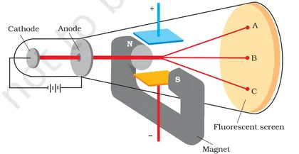
This chapter introduces the historical development and modern understanding of the atom — from early atomic models to the quantum mechanical model. It explains experimental evidence (cathode rays, scattering, spectra) that led to discovery of electron, proton and neutron and to successive models by Dalton, Thomson, Rutherford and Bohr. The chapter then develops the quantum description: de Broglie’s matter waves, Heisenberg uncertainty principle, Schrödinger wave equation (conceptual), and the interpretation of wavefunction leading to atomic orbitals. Key ideas include quantum numbers, shapes and energies of orbitals, electronic configuration rules (Aufbau, Pauli exclusion, Hund’s rule) and simple applications such as hydrogen spectrum, isotopes and isobars. Importance: understanding atomic structure is foundational for chemical bonding, periodicity and reactivity. What students will learn: how experimental observations shaped atomic models, why classical ideas failed, how quantum mechanics describes electron distribution, how to assign electronic configurations, and how atomic structure explains spectral lines and basic chemical properties.
Learning Objectives
- Define atomic number, mass number, isotopes and isobars and state their significance in describing atoms
- Explain Thomson's and Rutherford's atomic models, citing the experiments that supported them and their limitations
- Describe the alpha-particle (Rutherford) scattering experiment and deduce conclusions about nuclear structure
- State Bohr's postulates and apply them to derive expressions for the energy levels of hydrogen-like (one-electron) atoms
- Calculate wavelengths and frequencies of spectral lines using the Rydberg formula and Bohr model results
- Explain wave-particle duality and use the de Broglie relation to calculate the wavelength of moving particles
- State Heisenberg's uncertainty principle and solve simple problems involving position–momentum uncertainty
- Explain qualitatively the significance of the Schrödinger wave equation and interpret the physical meaning of the wavefunction and probability density
Topics in this chapter
17 topics · tap a topic title to jump straight to it.
Historical development of atomic theory
Overview and timeline
- John Dalton (early 19th century): Dalton proposed that matter is made of indivisible atoms, each element consists of identical atoms with characteristic masses, and compounds form by combination of atoms in simple whole-number ratios. His ideas explained laws of conservation of mass, definite proportions and multiple proportions.
- J. J. Thomson (1897): Discovery of the electron by cathode-ray experiments showed atoms have internal structure. He measured charge-to-mass ratio (e/m) of the electron and proposed the 'plum pudding' model: electrons embedded in a diffuse positive charge.
- Robert A. Millikan (1909): Oil-drop experiment measured the elementary charge e, giving an absolute value for electron charge and enabling accurate electron mass from Thomson's e/m.
- Ernest Rutherford (1911): Gold foil (α-particle scattering) experiment revealed a small, dense, positively charged nucleus; most of the atom is empty space. Rutherford model: electrons orbit a compact nucleus, but classical mechanics could not explain stable orbits or line spectra.
- Niels Bohr (1913): Bohr introduced quantized orbits for the hydrogen atom. Postulates: electrons occupy fixed energy levels (En), emit/absorb photons when jumping between levels; angular momentum quantized as mvr = nħ. This explained hydrogen spectral lines (Balmer, Lyman series) and gave formulas for En and radii rn.
- de Broglie, Schrödinger & Heisenberg (1920s): quantum mechanics: de Broglie proposed wave nature of particles (λ = h/p). Schrödinger developed the wave equation (ψ), whose solutions give allowed energy levels and probability distributions (orbitals). Heisenberg formulated the uncertainty principle (Δx·Δp ≥ ħ/2). These replaced Bohr orbits by orbitals described by quantum numbers (n, l, m_l, m_s).
Key experiments and what they showed
- Cathode-ray tube: existence of electrons, charge-to-mass ratio.
- Oil-drop: absolute charge of electron.
- Alpha scattering (gold foil): tiny dense nucleus, mostly empty space.
- Spectral emission/absorption: quantized energy levels (Bohr) and later explained by wave mechanics.
From models to modern view
Dalton's indivisible atom → Thomson's internal structure (electrons) → Rutherford's nucleus → Bohr's quantized energy levels (good for H-like atoms) → quantum mechanics: electrons are described by wavefunctions (ψ), probabilities, and four quantum numbers. The modern atomic model explains chemical periodicity, bonding, spectra, magnetism and many technologies (spectroscopy, semiconductors, microscopy).
Important conceptual points for Class 11
- Atomic models evolved as new experimental data appeared; each model solved some problems but had limitations addressed by later theories.
- Bohr model is useful for simple hydrogen-like systems; quantum mechanics (Schrödinger + Pauli + spin) gives full description of multi-electron atoms.
- Sodium street lamps: characteristic yellow emission comes from electron transitions in sodium atoms (spectroscopy), illustrating quantized energy levels.
- Hydrogen discharge tube: visible spectral lines (Balmer series) are explained by Bohr energy level transitions.
- Electron microscope: uses wave nature of electrons (de Broglie wavelength) to achieve resolutions far beyond optical microscopes.
- Mass spectrometry: separation of isotopes and determination of atomic masses relies on charged-particle behavior established since Thomson and Millikan.
- Bohr energy levels (hydrogen-like): En = -13.6 eV * Z^2 / n^2
- Bohr radius (nth orbit): rn = n^2 * a0 / Z , where a0 = 0.529 × 10^-10 m
- Rydberg formula (spectral lines): 1/λ = R * Z^2 * (1/n1^2 - 1/n2^2), R = 1.097373 × 10^7 m^-1
- Photon energy-wavelength relation: ΔE = hc/λ (h = 6.626 × 10^-34 Js, c = 3.00 × 10^8 m/s)
- de Broglie relation: λ = h / p = h / (mv)
- Heisenberg uncertainty (standard form): Δx · Δp ≥ ħ / 2 , where ħ = h / (2π)
Discovery of subatomic particles
Overview: The atom was once thought indivisible. Experiments from the late 19th and early 20th centuries revealed three basic subatomic particles — electron, proton and neutron — and led to the nuclear model of the atom.
1. Discovery of electron (J. J. Thomson, 1897)
Experiment: Cathode-ray tube (CRT). A high voltage across electrodes in a partially evacuated tube produced a beam (cathode rays) that: (a) travelled in straight lines, (b) caused fluorescence on a screen, and (c) was deflected by electric and magnetic fields.
Key observations and conclusions:
- Deflection by electric/magnetic fields shows the rays are charged particles.
- All cathode rays had the same charge-to-mass ratio (e/m) independent of the cathode material, implying particles (later called electrons) are constituents of all atoms.
2. Charge and mass of electron (Millikan oil-drop experiment, 1909)
Experiment: Tiny charged oil drops were suspended between charged plates. By balancing gravitational and electric forces and using viscous drag corrections, Millikan measured the charge on many drops and found they were integer multiples of a smallest value (the elementary charge, e ≈ 1.602×10^−19 C). Combined with Thomson’s e/m, the electron mass m_e was obtained.
3. Discovery of positive particles (canal rays and hydrogen nucleus)
Experiment: Goldstein (1886) observed canal rays (anode rays) — positive ions moving opposite to cathode rays in specially designed tubes. Later studies showed one of these positive particles was the hydrogen ion (H+), a single-proton nucleus.
Conclusion: Atoms contain a positively charged particle (proton) with charge +e.
4. Nuclear model from alpha-particle scattering (Ernest Rutherford, 1909–1911)
Experiment: A beam of alpha particles was directed at a thin gold foil. Most passed through with little deflection, but a few were deflected at large angles, some even back-scattered.
Conclusions:
- Most of an atom is empty space (alpha particles pass through).
- There is a very small, massive, positively charged nucleus that causes large-angle deflections.
- The nuclear model replaced the uniform "plum-pudding" model.
5. Discovery of neutron (James Chadwick, 1932)
Experiment: Bombarding beryllium with alpha particles produced a neutral penetrating radiation which knocked protons out of paraffin. The properties of this radiation (no charge, mass similar to proton) indicated a neutral particle — the neutron.
Reaction used (example): 9Be + 4He → 12C + 1n
Summary of particle properties (qualitative):
- Electron: negative charge (−e), very small mass (m_e ≈ 9.11×10^−31 kg).
- Proton: positive charge (+e), mass ≈ 1.67×10^−27 kg.
- Neutron: neutral (0), mass ≈ 1.67×10^−27 kg (≈ proton mass).
Why these discoveries matter: They established that atoms are composite, led to the nuclear model and later quantum models, and form the basis of chemistry, nuclear physics and technologies like electronics, nuclear energy and medical imaging.
- Electrons: flow of electrons in wires produces electric current; electron beams in electron microscopes provide very high-resolution imaging.
- Protons: in proton-exchange membrane fuel cells hydrogen ions (protons) move through the membrane to produce electricity; proton therapy uses high-energy protons to target cancerous tumors.
- Neutrons: neutrons are used to initiate and sustain nuclear chain reactions in reactors and for neutron activation analysis/materials probing; neutron diffraction determines crystal structures of materials.
- Kinetic energy of accelerated charge: eV = (1/2) m v^2 (useful in Thomson/Millikan contexts)
- Thomson (combined E and B fields) method: when electric and magnetic deflections cancel, v = E/B. Then from circular motion in magnetic field: e/m = v/(B r) = E/(B^2 r)
- Thomson (using accelerating potential V and radius r in B): e/m = 2V/(B^2 r^2)
- Millikan (relation for charge on a drop): q = (4/3) π r^3 (ρ_oil − ρ_air) g · (d/V) (where d = plate separation, V = applied voltage; r determined from viscous-drag measurements)
- Rutherford scattering (angular dependence): scattered intensity ∝ 1 / sin^4(θ/2) (Rutherford differential cross-section shows strong forward-peaking and 1/sin^4(θ/2) dependence)
Thomson's model of atom
Context: After the discovery of the electron (J. J. Thomson, 1897) Thomson proposed a model of the atom (circa 1904) to explain how negative electrons could exist inside an electrically neutral atom.
Basic idea (Plum‑pudding model): The atom is a sphere of uniform positive charge in which electrons are embedded like plums in a pudding. The positive charge is spread over the whole volume so that the total positive charge balances the total negative charge of the electrons; the atom as a whole is electrically neutral.
Assumptions:
- The atom is a sphere of radius R containing uniformly distributed positive charge +Q.
- Electrons (each of charge −e and mass m_e) are embedded at fixed positions inside this positive sphere.
- Electrostatic forces between the smeared positive charge and the electrons provide forces that hold electrons in place.
- For small displacements of an electron from equilibrium the net force is restoring (simple harmonic motion around equilibrium).
Simple electrostatic consequence (field inside a uniformly charged sphere):
For a uniformly charged sphere (total +Q, radius R), electric field at a distance r (r < R)
E(r) = (1 / (4πε0)) * (Q_enclosed / r^2)
But Q_enclosed = Q * (r^3 / R^3)
So E(r) = (1 / (4πε0)) * (Q * r / R^3)
Force on an electron & SHM behaviour:
F = −e E(r) = − (1 / (4πε0)) * (Q e / R^3) * r
This is a restoring force proportional to displacement r, so an electron displaced slightly undergoes simple harmonic motion with
ω^2 = (1 / (4πε0)) * (Q e) / (m_e R^3)
If the atom is neutral and Q = Z e (Z = total positive charge in units of e),
ω^2 = (1 / (4πε0)) * (Z e^2) / (m_e R^3)
Merits of Thomson's model:
- Explained electrical neutrality of atoms and existence of electrons as constituents.
- Provided a physical picture in which electrons could be in stable equilibrium (oscillatory motion) within the positive charge distribution.
- Was an important historical step toward more accurate models.
Limitations (why it was replaced):
- Could not explain the results of alpha‑particle scattering (Geiger–Marsden experiments) which showed a concentrated positive nucleus (Rutherford, 1911).
- Could not account for atomic spectral lines (discrete emission spectra) or chemical behavior dependent on nuclear charge and electron arrangement.
- The assumption of a continuous positive charge cloud has no experimental support; model gives incorrect scattering predictions and wrong spatial distribution of mass/charge.
Conclusion: Thomson's model (plum‑pudding) was a useful early attempt to place electrons inside atoms and to explain neutrality, but it failed quantitatively for scattering and spectral phenomena, and was superseded by Rutherford's nuclear model and later by Bohr and quantum models.
- Analogy: A chocolate chip cookie (or plum pudding) — the dough represents the positive charge spread out, and the chocolate chips are electrons embedded in it.
- Teaching example: Use a hollow transparent sphere filled with colored gelatin (positive charge) with beads (electrons) set into it to visualise embedded electrons.
- Experimental contrast: Rutherford’s gold‑foil experiment is a real‑life experiment that disproved the plum‑pudding picture — most alpha particles passed through but some were strongly deflected, implying a small dense positive nucleus (not a diffuse positive cloud).
- Coulomb constant: k = 1 / (4πε0).
- Electric field inside uniformly charged sphere (r < R): E(r) = (1 / (4πε0)) * (Q * r / R^3).
- Force on an electron at displacement r: F = −e E(r) = −(1 / (4πε0)) * (Q e / R^3) * r.
- Angular frequency of small oscillations: ω^2 = (1 / (4πε0)) * (Q e) / (m_e R^3). For a neutral atom with Q = Z e: ω^2 = (1 / (4πε0)) * (Z e^2) / (m_e R^3).
- Period of oscillation: T = 2π * sqrt( m_e R^3 / ( (1/(4πε0)) Z e^2 ) ).
Rutherford's nuclear model
Introduction: Rutherford's nuclear model (1911) replaced the plum‑pudding view of the atom and established that most of an atom's mass and all its positive charge are concentrated in a very small central nucleus, while electrons move around this nucleus in largely empty space.
Gold‑foil (alpha scattering) experiment — setup: A narrow beam of alpha (α) particles from a radioactive source was directed at a very thin gold foil. A circular fluorescent screen around the foil detected scattered α particles. Observations of scattering angles and counts led to key conclusions.
Key observations:
- Most α particles passed straight through the foil with little or no deflection (atom is mostly empty space).
- A small fraction were deflected through large angles (strong localized repulsive force).
- Very few (~1 in 20,000) were deflected back nearly 180° (center is very small and very dense).
Conclusions / Postulates of Rutherford's model:
- All positive charge and almost all mass of an atom are concentrated in a tiny central nucleus whose radius is on the order of 10^(-15) m.
- The nucleus carries a positive charge equal to Ze (Z = atomic number), where e is the elementary charge.
- Electrons move around the nucleus occupying the remaining space; most of the atom is empty space.
- Deflection of charged projectiles is due to Coulomb (electrostatic) repulsion between the positively charged nucleus and the incoming positively charged particles.
Physical picture & significance: The atom is not a uniform sphere of charge. Instead, a tiny dense nucleus (protons + neutrons, discovered later) is surrounded by electrons. Rutherford's model explained scattering data and laid the foundation for later quantum models (Bohr, wave mechanics) and nuclear physics.
Limitations: Rutherford's model could not explain the stability of orbiting electrons (classical electrodynamics predicts spiralling into the nucleus due to radiation) nor discrete atomic spectra. These problems were later resolved by Bohr's postulates and quantum mechanics.
Experimental & modern relevance: Rutherford scattering principles are used today in material analysis (Rutherford backscattering spectrometry), particle accelerators and detectors to probe nuclear and subnuclear structure, and underpin our understanding of nuclear reactions, radioactivity, and applications in medicine and energy.
- Gold‑foil experiment (Rutherford's original experiment) — demonstration that atoms are mostly empty space with a small dense nucleus.
- Rutherford backscattering spectrometry (RBS) — a modern technique that uses backscattered ions to analyze thin films and surface composition.
- Particle scattering experiments in accelerators (e.g., probing nuclei and substructure) — the same scattering principles are scaled to higher energies.
- Nuclear applications (reactors, medical radioisotopes) — rely on the concept of a concentrated atomic nucleus and its reactions.
- Coulomb (electrostatic) force between two point charges: F = (1/(4πε₀)) * (Z1 Z2 e²) / r², where Z1, Z2 are charge numbers, e is elementary charge, r is separation, ε₀ is vacuum permittivity.
- Closest approach (head‑on collision) from energy conservation: r_min = (1/(4πε₀)) * (Z1 Z2 e²) / E, where E is kinetic energy of the incoming charged particle.
- Rutherford differential scattering cross section (angular distribution): dσ/dΩ = [ (1/(4πε₀))² * (Z1 Z2 e²)² ] / [ 16 E² * sin⁴(θ/2) ], where θ is the scattering angle and E is the kinetic energy of the incident particle. (This predicts the 1/sin⁴(θ/2) dependence of scattering intensity.)
Bohr model of hydrogen atom
Overview: The Bohr model (Niels Bohr, 1913) explains the hydrogen atom spectra by combining classical mechanics with a quantum postulate: electrons move in certain allowed circular orbits without radiating energy and can jump between these orbits by absorbing or emitting a photon.
Bohr's postulates (concise):
- Electrons revolve in circular orbits about the nucleus under Coulomb attraction. Only certain orbits (stationary states) are allowed.
- An electron in an allowed orbit has a fixed energy and does not emit radiation.
- Angular momentum is quantized: m v r = nħ, where n = 1, 2, 3, ... (ħ = h/2π).
- Radiation is emitted/absorbed when an electron jumps between allowed orbits. The photon energy equals the energy difference: ΔE = hν.
Derivation (key steps):
- For a hydrogen-like atom (nucleus charge +Ze), equate Coulomb force to centripetal force: (1/4πε0) (Ze e)2 / r2 = m v2 / r.
- Use quantization m v r = nħ to eliminate v and solve for orbit radius rn:
rn = a0 (n2/Z), where a0 = 4πε0 ħ2 / (m e2) ≈ 0.529 × 10⁻¹⁰ m (Bohr radius).
Energy of level n:
En = - (me e4 Z2) / (8 ε02 h2 n2) = -13.6 eV × (Z2/n2) (for hydrogen Z = 1). Ground state (n=1) E1 = -13.6 eV.
Spectral lines (Rydberg formula):
When an electron falls from level ni to nf (ni > nf), the emitted photon has energy ΔE = Ei - Ef = hν = hc/λ. This leads to
1/λ = RH (1/nf2 - 1/ni2), where RH ≈ 1.097373 × 10⁷ m-1 (Rydberg constant for hydrogen).
Successes: Explains the hydrogen emission lines quantitatively (Balmer, Lyman, Paschen series), predicts ionization energy and radii, and works well for hydrogen-like (single-electron) ions such as He+, Li2+.
Limitations: Cannot explain fine structure, Zeeman effect, or spectra of multi-electron atoms; incompatible with the wave nature of electrons (replaced by quantum mechanics / Schrödinger model). Bohr's angular-momentum quantization is ad hoc; Schrödinger's wave mechanics gives deeper justification.
Practical notes: In CBSE Class 11 problems you'll often compute rn, En, wavelengths for transitions, and use n values for series identification (e.g., Balmer: nf = 2 produces visible lines).
- Hydrogen discharge tube: when hydrogen gas is excited in a discharge tube it emits visible spectral lines (Balmer series). The prominent H-α line is at 656 nm (transition n = 3 → n = 2).
- Astronomy: H-α and other hydrogen lines are used to identify hydrogen in stellar spectra and to study star-forming regions (H II regions).
- Hydrogen-like ions: He⁺ and Li²⁺ show spectral lines predicted by Bohr formula when Z>1 (energy levels scale as Z²).
- Ionization energy calculations: the ionization energy of H from ground state is 13.6 eV (energy required to remove the electron, n = 1 → ∞).
- Quantization of angular momentum: m v r = n ħ (n = 1, 2, 3, ...)
- Bohr radius: r_n = a_0 (n^2 / Z), where a_0 = 4πε_0 ħ^2 / (m e^2) ≈ 0.529 × 10^-10 m
- Energy of nth level: E_n = -13.6 eV × (Z^2 / n^2) (for hydrogen Z = 1). In SI: E_n = - (m e^4 Z^2) / (8 ε_0^2 h^2 n^2)
- Photon energy for transition: ΔE = E_i - E_f = h ν = hc / λ
- Rydberg formula: 1/λ = R_H (1/n_f^2 - 1/n_i^2), where R_H ≈ 1.097373 × 10^7 m^-1
- Ground state energy (n=1): E_1 = -13.6 eV = -2.18 × 10^-18 J
Atomic spectra
What are atomic spectra?
Atomic spectra are patterns of electromagnetic radiation (light) emitted or absorbed by atoms. They occur because electrons in atoms occupy discrete (quantized) energy levels; when an electron moves between levels it absorbs or emits a photon whose energy equals the difference between the two levels. Atomic spectra are characteristic of each element and are used to identify elements.
Types of spectra
- Continuous spectrum: Emitted by hot dense bodies (filament, blackbody). All wavelengths appear as a continuous band.
- Emission (line) spectrum: Bright lines on dark background. Produced by atoms in low-pressure gas discharged or excited — each bright line corresponds to a specific transition.
- Absorption spectrum: Dark lines on a continuous background. When continuous radiation passes through a cooler gas, photons of specific energies are absorbed corresponding to allowed transitions.
Bohr model explanation (for hydrogen-like atoms)
Key ideas (Bohr postulates): electrons move in certain allowed circular orbits without radiating; each orbit has quantized energy E_n; emission/absorption occurs when an electron jumps between orbits. For hydrogen, the energy of the nth level is given by E_n = -13.6 eV / n^2 (or E_n = -2.18 × 10⁻¹⁸ J / n^2). The photon energy for a transition from n_i to n_f is ΔE = E_i - E_f = hν = hc/λ.
Rydberg formula (wavelengths of hydrogen spectral lines)
For hydrogen-like atoms, the wavelengths of spectral lines are given by the Rydberg formula:
1/λ = R_H (1/n_f^2 - 1/n_i^2), with n_i > n_f. Here R_H is the Rydberg constant for hydrogen ≈ 1.097373 × 10⁷ m-1.
Important spectral series for hydrogen
- Lyman series: n_f = 1 (ultraviolet)
- Balmer series: n_f = 2 (visible; e.g., Hα = 656.3 nm)
- Paschen series: n_f = 3 (infrared)
Other series include Brackett (n_f = 4), Pfund (n_f = 5), etc.
Why spectra are useful (applications)
Identification of elements (flame tests, atomic emission spectroscopy), astrophysics (Fraunhofer lines in solar spectrum reveal elemental composition and physical conditions in stars), neon and sodium street lights, lasers (population inversion and stimulated emission), and analytical chemistry (qualitative and quantitative analysis).
Additional notes
- Absorption and emission lines for the same transitions occur at the same wavelengths (emission bright lines correspond to absorption dark lines at same λ).
- Real spectra show line broadening (Doppler, pressure, instrumental) and fine/hyperfine structures due to electron spin, relativistic effects and nuclear interactions.
- Selection rule (electric-dipole): Δl = ±1 usually governs allowed transitions (where l is orbital quantum number).
- Neon signs: different gases/mixtures emit characteristic coloured line spectra when electrically excited.
- Sodium street lamps: intense yellow emission at ≈589 nm due to sodium D-lines (used for lighting).
- Flame tests in qualitative analysis: copper gives green, lithium gives crimson — due to element-specific emission lines.
- Solar (Fraunhofer) lines: dark absorption lines in sunlight identify elements in the Sun's atmosphere and indicate motions (Doppler shifts).
- Astronomical spectroscopy: redshift of galaxy spectral lines (change in observed λ) used to measure velocity and expansion of the universe.
- E_n = -13.6 eV / n^2 (Hydrogen energy levels) = -2.18 × 10^-18 J / n^2
- ΔE = E_i - E_f = hν = hc/λ
- Rydberg formula: 1/λ = R_H (1/n_f^2 - 1/n_i^2), R_H = 1.097373 × 10^7 m^-1
- Photon energy–wavelength relation: E = hc/λ, with h = 6.626 × 10^-34 J·s, c = 3.00 × 10^8 m/s
- Energy of ground state (n=1): E_1 = -13.6 eV (for hydrogen)
Quantum nature of radiation
Introduction
The quantum nature of radiation means that electromagnetic radiation is not only a continuous wave but also exists as discrete packets of energy called photons. This idea explains phenomena that classical wave theory could not, such as blackbody radiation and the photoelectric effect.
Historical background and why quantum idea arose
- Blackbody radiation: Classical theories (Rayleigh–Jeans law) predicted infinite energy at short wavelengths (the ultraviolet catastrophe).
- Planck's hypothesis (1900): To resolve this, Planck proposed that energy exchange between matter and electromagnetic field occurs in discrete amounts. A harmonic oscillator (emitter/absorber) can have energies E = n h ν (n = 0,1,2,...), where h is Planck's constant and ν is frequency.
- Einstein and photons (1905): Einstein extended Planck's idea to light itself, proposing that light consists of quanta (photons) each with energy E = h ν. This explained the photoelectric effect and established the particle aspect of light.
Key consequences and evidences
- Photoelectric effect: Electrons are ejected from a metal when struck by light only if the light frequency exceeds a threshold ν0. The maximum kinetic energy of ejected electrons depends on frequency, not intensity. This matches Einstein's equation KEmax = hν − φ (φ = work function).
- Discrete spectra: Atoms emit light at specific wavelengths (line spectra). Each emitted photon corresponds to an energy difference between atomic energy levels ΔE = hν.
- Compton effect: X‑ray scattering from electrons shows a wavelength shift consistent with treating X‑rays as particles with momentum p = h/λ, supporting particle properties of radiation.
Summary of the physical picture
Radiation shows wave properties (interference, diffraction) and particle properties (photoelectric effect, Compton scattering). The quantum view: electromagnetic radiation is quantized into photons of energy E = hν and momentum p = h/λ. Energy exchange between light and matter occurs in integral multiples of hν.
Practical importance
Understanding the quantum nature of radiation is fundamental to devices such as photovoltaic cells, photo-detectors, LEDs and lasers, and to techniques like X‑ray scattering and spectroscopy.
- Solar cells (photovoltaic panels): photons with E ≥ work function knock out electrons and generate current — application of the photoelectric principle.
- Photoelectric sensors and photomultiplier tubes: detection of individual photons or their effect on electrons.
- LEDs and lasers: emission of photons when electrons transition between energy levels in semiconductors or atoms.
- Compton scattering in medical X‑ray diagnostics: scattering demonstrates particle momentum of photons.
- Incandescent bulbs vs LEDs: incandescent bulbs approximate blackbody radiation (continuous spectrum), LEDs emit narrow-band (quantized) photons.
- Energy of a photon: E = h·ν (where h = 6.626×10⁻³⁴ J·s, ν = frequency in s⁻¹)
- Relation between frequency and wavelength: c = λ·ν (c = 2.998×10⁸ m·s⁻¹)
- Photon energy in terms of wavelength: E = h·c / λ
- Planck's quantization for oscillators: E_n = n·h·ν (n = 0,1,2,...)
- Einstein photoelectric equation: KE_max = h·ν − φ (φ = work function in J)
- Work function and threshold frequency: φ = h·ν₀ ⇒ ν₀ = φ / h
Wave–particle duality
Definition: Wave–particle duality is the concept that microscopic entities (light and matter) exhibit both wave-like and particle-like properties depending on the experiment and how they are observed. This idea unifies phenomena such as interference/diffraction (wave behaviour) and photoelectric/Compton effects (particle behaviour).
Historical basis: In the early 20th century Planck and Einstein treated light as quantized energy packets (photons) to explain blackbody radiation and the photoelectric effect. In 1924 Louis de Broglie proposed that material particles (electrons, neutrons, atoms) also have wave properties, characterized by a wavelength. Experiments (Davisson–Germer electron diffraction, electron double‑slit interference) later confirmed de Broglie’s hypothesis.
Key ideas and physical meaning:
- For photons: energy E and momentum p are related to frequency (ν) and wavelength (λ) by E = hν and p = h/λ (h = Planck’s constant). Photons act like particles with quantized energy and momentum, explaining photoelectric and Compton effects.
- For matter waves (de Broglie hypothesis): every particle of momentum p has an associated wavelength λ = h/p. For a non-relativistic particle p = mv, so λ = h/(mv). The wave character becomes significant when λ is comparable to the characteristic size (e.g., atomic spacing in crystals).
- Complementarity (Bohr): whether an entity shows wave or particle behaviour depends on the measurement setup. Both descriptions are needed for a full quantum picture.
Typical derivations (non-relativistic):
- De Broglie wavelength: λ = h/p. If p = mv (non-relativistic), λ = h/(mv).
- If an electron is accelerated through a potential difference V (so kinetic energy KE = eV), then p = sqrt(2m e V) and
λ = h / sqrt(2 m e V).
When is wave nature observable? For macroscopic objects the de Broglie wavelength is extraordinarily small (practically zero), so classical particle behaviour dominates. For electrons, neutrons, atoms, or molecules at typical laboratory energies, λ can be comparable to atomic spacings and diffraction/interference experiments reveal wave properties.
Experimental confirmations (brief):
- Photoelectric effect (Einstein): light behaves like particles (photons) delivering energy hv to eject electrons; supports quantization of light.
- Compton effect: X‑ray scattering from electrons shows wavelength shift consistent with photon momentum transfer (particle nature of light).
- Davisson–Germer experiment: electrons scattered from a crystal show diffraction peaks, proving electrons have wave nature with wavelength equal to de Broglie wavelength.
- Electron double‑slit experiments: single electrons build up an interference pattern—each electron shows both particle arrival and underlying wave interference.
Limitations & remarks: De Broglie hypothesis is part of non-relativistic quantum mechanics; for very high speeds (relativistic) use relativistic relations (p = γmv, E^2 = (pc)^2 + (mc^2)^2). Quantum mechanics replaces classical trajectories with probability amplitudes (wavefunctions) whose squared magnitude gives detection probabilities.
- Davisson–Germer electron diffraction: electrons scattered by a Ni crystal produce diffraction peaks — direct evidence of electron wave behaviour.
- Electron microscopes (TEM/SEM): use short de Broglie wavelengths of electrons to achieve much higher resolution than optical microscopes.
- Photoelectric effect in solar cells and photodiodes: light behaves like photons ejecting charge carriers; energy threshold depends on frequency.
- Compton scattering in X‑ray/gamma detectors: photon wavelength shifts after colliding with electrons, showing photon momentum.
- Neutron diffraction used to study crystal and magnetic structures: neutrons (matter waves) diffract from atomic planes similar to X‑rays.
- Planck relation: E = hν (E = energy, ν = frequency, h = 6.626 × 10⁻³⁴ J·s)
- Photon momentum: p = h/λ (also p = E/c for photons)
- De Broglie wavelength: λ = h/p
- Non‑relativistic particle: λ = h/(mv) where m = mass, v = velocity
- For a particle with kinetic energy KE (non‑relativistic): λ = h / sqrt(2 m KE)
- Electron accelerated through potential V: λ = h / sqrt(2 m_e e V) (m_e = 9.109 × 10⁻³¹ kg, e = 1.602 × 10⁻¹⁹ C)
Heisenberg uncertainty principle
Definition: The Heisenberg uncertainty principle (1927) states that certain pairs of physical properties (conjugate variables) cannot be simultaneously measured with arbitrary precision. For position x and momentum p the relation is: Δx · Δp ≥ ħ/2, where ħ = h/2π. This is a fundamental property of quantum systems, not a limitation of instruments.
Why it occurs: Particles behave as waves (wave–particle duality). A well localized wave (small Δx) requires the superposition of many momentum (wavelength) components, so the spread in momentum (Δp) becomes large. Mathematically this follows from properties of Fourier transforms: a narrow function in x-space corresponds to a broad function in p-space.
Consequences and interpretation for Class 11: Electrons in atoms cannot have simultaneously exact position and momentum—this is why we describe electrons by orbitals (probability distributions), not definite classical trajectories. The uncertainty principle explains the stability of atoms (zero-point motion), quantum tunnelling, and limits on measurement at very small scales. For macroscopic objects, Δx and Δp values make the product negligible compared to ħ, so classical physics applies.
Energy–time form: ΔE · Δt ≥ ħ/2. This relates the uncertainty in energy to the time interval over which the energy measurement is made (used to explain natural linewidth of spectral lines and short-lived excited states).
- Electron localization: If an electron is confined to about 1 × 10^−10 m (≈ atomic size), the minimum momentum uncertainty is Δp ≥ ħ/(2Δx) ≈ 1.05×10^−34/(2×10^−10) ≈ 5.3×10^−25 kg·m/s. For an electron (m = 9.11×10^−31 kg) this gives Δv ≈ 5.8×10^5 m/s, showing large velocity uncertainty for strong position localization.
- Scanning tunnelling microscope (STM): STM works because electrons can tunnel through a barrier; tunnelling probability depends on the wave nature and the uncertainty in position/momentum — a strictly classical particle picture would forbid tunnelling.
- Electron microscope resolution limit: Increasing electron beam localization increases momentum spread, affecting beam focusing and resolution—quantum limits influence ultimate resolution.
- Spectral line broadening: Short-lived excited states (small Δt) have uncertain energy (large ΔE), producing a natural linewidth of emitted spectral lines (energy–time uncertainty).
- Quantum tunnelling in semiconductors: Tunnel diodes and flash memory rely on electron tunnelling, which is explained by wavefunctions and the uncertainty principle rather than classical trajectories.
- Atomic orbitals: Electrons occupy orbitals (probability clouds). If we tried to confine an electron very close to the nucleus (small Δx), the large Δp would give large kinetic energy, preventing collapse — this helps explain atomic stability.
- Position–momentum uncertainty: Δx · Δp ≥ ħ/2 (where ħ = h/2π)
- Planck relation between momentum and wavelength: p = h/λ (connects wave character to momentum)
- Energy–time uncertainty: ΔE · Δt ≥ ħ/2
- Minimum uncertainty Gaussian wavepacket (example): For ψ(x) ∝ exp(−x^2/(4σ_x^2)), Δx = σ_x and Δp = ħ/(2σ_x), so Δx·Δp = ħ/2 (the minimum possible product).
Schrödinger wave equation and quantum mechanics
Overview
The Schrödinger wave equation is the core mathematical statement of non-relativistic quantum mechanics. It describes how the quantum state of a particle (or system) changes in space and time. The solution is a complex function called the wavefunction, Ψ (psi), whose square modulus gives the probability density of finding the particle at a point in space.
Wavefunction and its meaning
Ψ(x,y,z,t) is the wavefunction. It can be complex. The physically measurable quantity is the probability density, given by |Ψ|² = Ψ*Ψ (Born interpretation). For a single particle the normalization condition is ∫|Ψ|² dτ = 1 over all space.
Time-dependent Schrödinger equation
The fundamental equation (time-dependent) is:
iħ ∂Ψ/∂t = −(ħ²/2m) ∇²Ψ + V(r,t) Ψ
Here ħ = h/2π, m is the particle mass, ∇² is the Laplacian operator and V(r,t) is the potential energy.
Time-independent Schrödinger equation
For a time-independent potential, solutions can be separated as Ψ(r,t) = ψ(r)·T(t). The spatial part satisfies the time-independent (stationary) equation:
−(ħ²/2m) ∇²ψ + V(r) ψ = E ψ
where E is the energy eigenvalue. These ψ(r) are stationary states (energy eigenfunctions).
Operators and expectation values
Physical observables correspond to operators. Examples:
• Momentum operator: p̂ = −iħ ∇
• Hamiltonian (energy) operator: Ĥ = −(ħ²/2m) ∇² + V(r)
Expectation value of observable A with operator Â: <A> = ∫ψ* Â ψ dτ.
Quantization and boundary conditions
Only those ψ that satisfy the Schrödinger equation and appropriate boundary conditions (finite, single-valued, continuous) are allowed. These conditions lead to discrete allowed energies (quantization). For example, a particle in a 1D infinite box of length L has energy levels E_n ∝ n² (n = 1,2,3...).
Quantum numbers (for hydrogen-like atoms)
Solving the Schrödinger equation for the hydrogen atom yields wavefunctions characterized by quantum numbers: principal (n), azimuthal (l), magnetic (m_l) and spin (m_s). These determine energy (mainly n for hydrogen), shape (l), orientation (m_l) and intrinsic spin (m_s = ±1/2).
Heisenberg uncertainty principle
Quantum mechanics implies limits on simultaneous knowledge of conjugate variables. For position x and momentum p: Δx · Δp ≥ ħ/2. This is a fundamental property, not due to measurement faults.
Nodes and probability distributions
Wavefunctions can have nodes (points or surfaces where ψ = 0). |ψ|² gives the probability distribution. For hydrogen, radial and angular nodes determine where electrons are likely or unlikely to be found. Orbitals (s, p, d...) are shapes of constant probability regions.
Why it matters (conceptual)
Schrödinger equation replaces classical trajectories with probability amplitudes. Particles show wave-like behavior (diffraction, interference) captured by Ψ and particle-like behavior in measurements (discrete detection events). This duality explains atomic spectra, chemical bonding, tunneling, and many microscopic phenomena.
- Electron microscope: Uses the wave nature of electrons (short de Broglie wavelength) to achieve very high spatial resolution; design relies on understanding electron wave behavior and interactions.
- Scanning tunneling microscope (STM): Operates by quantum tunneling of electrons between a tip and sample; tunneling probability comes from solutions of the Schrödinger equation across a potential barrier.
- Semiconductor devices and LEDs: Electron energy levels, band structure and carrier behavior are explained by quantum mechanics; allowed and forbidden energy ranges determine electrical/optical properties.
- Alpha decay and quantum tunneling: Alpha particles escape a nucleus by tunneling through a potential barrier — a purely quantum effect predicted by wave mechanics.
- de Broglie relation: λ = h / p
- Time-dependent Schrödinger equation: iħ ∂Ψ/∂t = −(ħ² / 2m) ∇²Ψ + V(r,t) Ψ
- Time-independent Schrödinger equation: −(ħ² / 2m) ∇²ψ + V(r) ψ = E ψ
- Normalization: ∫ |ψ|² dτ = 1
- Probability density: P(r,t) = |Ψ(r,t)|² = Ψ*(r,t) Ψ(r,t)
- Momentum operator: p̂ = −iħ ∇
Quantum numbers and orbitals
Overview
Quantum numbers are a set of four numbers that describe the allowed states (orbitals) of electrons in an atom. Orbitals are regions in space where the probability of finding an electron is high. The four quantum numbers — principal (n), azimuthal or angular momentum (l), magnetic (ml) and spin (ms) — together uniquely identify an electron in an atom.
1. Principal quantum number (n)
- Denotes the main energy level or shell: n = 1, 2, 3, ...
- Gives approximate size and energy of the orbital. Higher n → larger orbital and typically higher energy.
- Maximum number of orbitals in a shell = n2. Maximum electrons in a shell = 2n2.
2. Azimuthal (angular momentum) quantum number (l)
- Determines shape of orbital and subshell type. For a given n, l = 0, 1, 2, ..., n−1.
- Subshell labels: l = 0 → s, 1 → p, 2 → d, 3 → f.
- Number of orbitals in a subshell = 2l + 1.
3. Magnetic quantum number (ml)
- Describes orientation of an orbital in space: ml = −l, −l+1, ..., 0, ..., +l.
- Each ml value corresponds to one orbital within a subshell.
4. Spin quantum number (ms)
- Represents intrinsic spin of the electron; possible values +1/2 or −1/2.
- Pauli exclusion principle: no two electrons in an atom can have the same set of all four quantum numbers.
Orbital shapes and nodes
- s orbitals (l = 0): spherical; probability density depends only on distance from nucleus.
- p orbitals (l = 1): dumbbell-shaped with a nodal plane at the nucleus; three orientations (px, py, pz), corresponding to ml = −1, 0, +1.
- d orbitals (l = 2): cloverleaf shapes (four lobes) for most; one (dz2) has a doughnut/torus shape around z-axis.
- Number of angular nodes = l. Number of radial nodes = n − l − 1. Total nodes = n − 1.
Energy and degeneracy
- For hydrogen-like (single-electron) atoms, energy depends only on n: En = −13.6 eV * Z2 / n2 (Z = nuclear charge).
- In multi-electron atoms, energies also depend on l due to electron-electron interactions; subshells split (e.g., 2s and 2p differ in energy).
Rules for filling electrons
- Aufbau principle: electrons occupy the lowest available energy orbitals first (order: 1s < 2s < 2p < 3s < 3p < 4s < 3d ... with common crossovers).
- Pauli exclusion principle: max two electrons per orbital with opposite spins.
- Hund’s rule: electrons occupy degenerate orbitals singly with parallel spins before pairing.
Notation and examples
- Orbital notation: 3p, 4d, etc. Electronic configuration example: O (Z = 8) → 1s2 2s2 2p4.
- Calculation example: For n = 3: allowed l = 0,1,2 (3s, 3p, 3d). Orbitals = n2 = 9 orbitals; maximum electrons = 2n2 = 18 electrons.
Quantum mechanical picture
- Orbitals are solutions (wavefunctions ψ) of the Schrödinger equation. The observable probability density is |ψ|2. Nodes are regions where ψ = 0 and |ψ|2 = 0.
- The quantum numbers arise naturally from boundary conditions on these wavefunctions.
Key takeaways for Class 11
- Four quantum numbers (n, l, ml, ms) uniquely describe an electron.
- Orbital shapes (s, p, d) and nodes explain geometry and many chemical properties.
- Simple formulae (n2, 2n2, 2(2l+1), radial nodes = n−l−1) help count orbitals/electrons.
- Counting orbitals: For n = 4, number of orbitals = n^2 = 16 and maximum electrons = 2n^2 = 32.
- Node count: For a 3p orbital (n = 3, l = 1): angular nodes = l = 1, radial nodes = n − l − 1 = 1, total nodes = 2.
- Electron configuration: Carbon (Z = 6) → 1s^2 2s^2 2p^2. According to Hund’s rule, the two 2p electrons occupy separate 2p orbitals with parallel spins.
- Spectroscopy application: Electron spin and orbital splitting under magnetic fields form the basis of Electron Spin Resonance (ESR) spectroscopy which probes unpaired electrons in radicals and transition metal complexes.
- Chemistry application: Colors of many transition-metal complexes arise from d-orbital splitting (crystal-field splitting) and electronic transitions between these split d-levels.
- Principal quantum number: n = 1, 2, 3, ...
- Azimuthal quantum number: l = 0, 1, 2, ..., (n−1) (labels: 0→s, 1→p, 2→d, 3→f)
- Magnetic quantum number: m_l = −l, −l+1, ..., 0, ..., +l
- Spin quantum number: m_s = +1/2 or −1/2
- Orbitals per shell = n^2
- Maximum electrons per shell = 2 n^2
Shapes of atomic orbitals
Overview
Atomic orbitals are regions in space around an atomic nucleus where the probability of finding an electron is high. The shape of an orbital is determined by the angular part of the wavefunction and depends on the quantum numbers (n, l, m_l). Orbital shapes explain atomic bonding, molecular geometry and many chemical properties.
Quantum numbers and general form
- Principal quantum number n = 1, 2, 3, ... — energy/shell.
- Azimuthal (angular) quantum number l = 0, 1, ..., n-1 — orbital type/shape: l = 0 (s), 1 (p), 2 (d), 3 (f).
- Magnetic quantum number m_l = -l, ..., 0, ..., +l — orientation (2l+1 values).
The general hydrogen-like orbital wavefunction is written as:
ψ_{n,l,m}(r, θ, φ) = R_{n,l}(r) · Y_{l}^{m}(θ, φ)
R_{n,l}(r) is the radial part (depends on r, n, l). Y_{l}^{m}(θ, φ) are spherical harmonics (determine the angular shape).
Nodes
- Total number of nodes = n − 1.
- Angular nodes = l (planes or cones where ψ = 0, e.g., p orbitals have 1 nodal plane).
- Radial nodes = n − l − 1 (spherical shells where radial part changes sign).
Shapes of common orbitals
- s-orbitals (l = 0): Spherically symmetric about the nucleus. Probability depends only on r. 1s is a single lobe with maximum at r > 0; higher ns have spherical radial nodes (shells).
- p-orbitals (l = 1): Dumbbell-shaped with two lobes of opposite phase separated by a nodal plane through the nucleus. Three orientations: p_x, p_y, p_z (m_l = −1, 0, +1).
- d-orbitals (l = 2): More complex: four of them have cloverleaf shapes (d_xy, d_yz, d_zx, d_x2−y2) and one (d_z2) has a donut (toroid) around the z-axis plus two lobes on z-axis. They have 2 angular nodes.
- f-orbitals (l = 3): Even more complex multi-lobed shapes used mainly in lanthanides and actinides.
Probability and radial distribution
Electron probability density at a point: |ψ|^2. Radial distribution function (probability of finding electron between r and r+dr): P(r) = 4π r^2 |R_{n,l}(r)|^2. Peaks in P(r) correspond to most probable radii (shells).
Why shapes matter (chemical consequences)
- Directional character of p and d orbitals explains directional bonding (e.g., π-bonds from sidewise overlap of p orbitals).
- Hybridization (sp, sp2, sp3) uses combinations of s and p orbitals to produce directional bonds (e.g., tetrahedral CH4 uses sp3 hybrids).
- d-orbitals are central to transition-metal chemistry: bonding, magnetism and color (crystal-field splitting depends on d-orbital orientations).
Simple hydrogenic examples (functional forms, up to constant normalization)
- 1s: R_{1,0}(r) ∝ e^{−r/a_0} (spherical).
- 2s: R_{2,0}(r) ∝ (2 − r/a_0) e^{−r/(2a_0)} (has one radial node where 2 − r/a_0 = 0).
- 2p angular part: Y_{1}^{m}(θ,φ) ⇒ p lobes with a nodal plane; radial part R_{2,1}(r) ∝ r e^{−r/(2a_0)}.
Summary of counting rules
- Number of orbitals in shell n = n^2.
- Maximum electrons in shell n = 2n^2.
- Magnetic orientations per subshell l = 2l + 1.
Useful classroom remarks: Emphasize that orbitals are probability distributions (not classical orbits). The shapes are solutions of the Schrödinger equation for hydrogen-like atoms and remain a good qualitative guide for multi-electron atoms.
- Methane (CH4): Carbon uses sp3 hybrid orbitals (combining one 2s and three 2p orbitals) to form four equivalent tetrahedral bonds — demonstrates how atomic orbital shapes determine molecular geometry.
- Ethene (C2H4): Each carbon is sp2 hybridized; the unhybridized p orbital on each carbon overlaps side-by-side to form a π bond. The shape and orientation of p orbitals are essential for π bonding.
- Water (H2O): Oxygen’s two lone pairs occupy orbitals with directional character (roughly sp3-like), producing the bent molecular shape and bond angle (~104.5°).
- Transition-metal complexes: d-orbital orientations (d_xy, d_xz, d_yz, d_x2−y2, d_z2) interact differently with ligands giving crystal-field splitting; this controls color and magnetic properties of complexes.
- Scanning tunneling microscopy (STM): Measured electron density near surfaces reflects orbital shapes (e.g., imaging of s, p-like states on atoms or molecules).
- Organic conjugated systems (benzene): p orbitals perpendicular to the ring overlap to form delocalized π molecular orbitals, responsible for aromaticity and electronic absorption spectra.
- \[General wavefunction: ψ_{n,l,m}(r,θ,φ) = R_{n,l}(r) · Y_{l}^{m}(θ,φ)\]
- \[Probability density at a point: P(r,θ,φ) = |ψ_{n,l,m}(r,θ,φ)|^2\]
- \[Radial distribution function: RDF(r) = 4π r^2 |R_{n,l}(r)|^2 (probability of electron between r and r + dr)\]
- Node counts: total nodes = n − 1; angular nodes = l; radial nodes = n − l − 1
- Magnetic quantum number range: m_l = −l, −l+1, ..., 0, ..., +l (2l + 1 orientations)
- Orbitals per shell: number = n^2; maximum electrons per shell = 2 n^2
Electronic configuration
What is electronic configuration? Electronic configuration is the arrangement of electrons in the orbitals of an atom. It tells how electrons are distributed among different shells (energy levels), subshells (s, p, d, f) and orbitals according to quantum mechanics and governs chemical behavior.
Quantum numbers (brief):
- Principal quantum number n = 1,2,3,... (shell, energy, size)
- Azimuthal (angular) quantum number l = 0,...,n-1 (subshell: 0→s, 1→p, 2→d, 3→f)
- Magnetic quantum number ml = −l,...,0,...,+l (specific orbital)
- Spin quantum number ms = +1/2 or −1/2 (electron spin)
Rules for filling electrons:
- Aufbau principle: Electrons occupy orbitals of lowest energy first. Practically use (n + l) rule (Madelung rule); if (n + l) equal, lower n fills first.
- Pauli exclusion principle: No two electrons in an atom can have the same set of four quantum numbers — an orbital holds at most two electrons with opposite spins.
- Hund's rule: For degenerate orbitals (same energy), electrons occupy them singly with parallel spins before pairing.
Notation: Write shells/subshells with electron counts: e.g. 1s2, 2s22p6, etc. Use noble-gas shorthand: e.g. Fe = [Ar] 4s2 3d6.
Common exceptions (brief): Some transition metals show anomalous configurations for extra stability of half-filled or fully filled d subshells. Examples: Cr: [Ar] 4s1 3d5 (not 4s23d4), Cu: [Ar] 4s1 3d10.
Why it matters: Electronic configuration explains periodic properties (atomic size, ionization energy, valency), bonding, magnetism (unpaired electrons), color and spectra (electronic transitions) and chemical reactivity.
- H: 1s1
- He: 1s2
- C: 1s2 2s2 2p2 (valence 2s2 2p2 → four valence electrons)
- O: 1s2 2s2 2p4 (two unpaired electrons in 2p → paramagnetic)
- Na: 1s2 2s2 2p6 3s1 or [Ne] 3s1 (forms Na+ by losing 3s electron → [Ne])
- Cl: [Ne] 3s2 3p5 (gains one electron to become Cl− → [Ar])
- Maximum electrons in nth shell: 2n^2
- Maximum electrons in a subshell with quantum number l: 2(2l + 1) (e.g., s:2, p:6, d:10, f:14)
- Energy of hydrogen-like atom (approx.): E_n = -13.6 eV * (Z^2 / n^2) where Z = nuclear charge, n = principal quantum number
- Aufbau (Madelung) ordering rule: fill orbitals in increasing order of (n + l); if equal, lower n first
- Spin quantum number values: m_s = +1/2 or -1/2
Stability concepts and exceptions (basic)
Basic idea of stability
An atom (or ion) is especially stable when its electrons occupy energetically favourable arrangements. In simple terms, completely filled shells/subshells (noble‑gas configuration) and half‑filled subshells often give extra stability. Stability rules used in Class 11 are the Aufbau principle, Pauli exclusion principle and Hund's rule, together with the (n + l) rule for orbital filling order.
Why some arrangements are more stable
1. Completely filled subshells (e.g. p6, d10) are symmetric and have lower energy because there is maximum pairing and exchange stabilization.
2. Half‑filled subshells (e.g. p3, d5) are also relatively stable because of symmetry and maximum parallel spins which increases exchange energy and lowers the total energy.
3. For transition elements the energy difference between the (n)s and (n−1)d orbitals is very small. Small energy differences allow one electron to move from s to d to produce a half‑filled or filled d subshell, giving an anomalous (more stable) configuration.
Common exceptions (basic list)
Because of the small energy gap between ns and (n−1)d orbitals, some elements do not follow the simple Aufbau filling. Typical examples (ground state electronic configurations):
- Chromium (Cr): expected [Ar] 3d4 4s2 → actual [Ar] 3d5 4s1 (half‑filled d5 is more stable)
- Copper (Cu): expected [Ar] 3d9 4s2 → actual [Ar] 3d10 4s1 (filled d10 is more stable)
- Molybdenum (Mo): [Kr] 4d5 5s1 (d5 extra stability)
- Silver (Ag): [Kr] 4d10 5s1 (d10 extra stability)
- Palladium (Pd): expected [Kr] 4d8 5s2 → actual [Kr] 4d10 5s0 (complete d10 preferred)
Why these exceptions occur (qualitative)
- Exchange energy: parallel spins in different orbitals lower the energy (important for half‑filled subshells).
- Electron‑electron repulsion and orbital penetration: moving an electron from s to d can reduce repulsion or increase stability because d orbitals combine better with the existing occupation.
- Small differences in orbital energies (ns vs (n−1)d) make such rearrangements energetically favourable.
Ions and removal of electrons
For transition metals, although neutral atoms may have ns occupied, on ionization the ns electron(s) are lost first and then d electrons, because in ions (n−1)d lies lower in energy than ns. Example: Fe: ground state [Ar] 3d6 4s2, on forming Fe2+ → configuration [Ar] 3d6 (both 4s electrons removed).
Practical/CBSE focus
Students should be able to: state and apply Aufbau, Pauli, Hund rules; use (n + l) rule; write ground‑state configurations for first‑row transition metals and recognize the common Cr/Cu type exceptions; explain qualitatively why half‑filled and fully filled subshells are extra stable.
- Noble gases (He, Ne, Ar) are inert because they have completely filled shells (very stable).
- Chromium (Cr): actual configuration [Ar] 3d5 4s1 instead of expected 3d4 4s2 because half‑filled d5 is more stable.
- Copper (Cu): actual configuration [Ar] 3d10 4s1 instead of expected 3d9 4s2 because filled d10 is more stable.
- Formation of Fe2+: neutral Fe [Ar] 3d6 4s2 → Fe2+ becomes [Ar] 3d6 (4s electrons removed first).
- Palladium (Pd): ground state [Kr] 4d10 5s0 — shows a complete d10 subshell preference.
- n + l rule: orbitals with lower (n + l) fill first; if tie, lower n fills first (where n = principal quantum number, l = azimuthal quantum number).
- Hydrogen‑like energy (for reference): E_n = −13.6 Z^2 / n^2 eV (shows energy scale of levels for H‑like atoms).
- Magnetic moment (spin‑only) for paramagnetic species: μ = √[n(n + 2)] μ_B, where n = number of unpaired electrons and μ_B = Bohr magneton (used to relate unpaired electrons to observed magnetism).
Isotopes, isobars and isotones
Overview & notation
Atoms (nuclides) are specified by their atomic number Z (number of protons) and mass number A (total number of protons + neutrons). The conventional notation is AZX, where X is the chemical symbol, A is the mass number and Z is the atomic number. The neutron number N = A − Z.
Isotopes
Definition: Isotopes are nuclides of the same element (same Z) but with different mass numbers A (different N). They have identical chemical properties (same electron configuration) but may show different physical or nuclear properties (e.g., different stability, radioactive behaviour).
Examples and key points:
- Hydrogen isotopes: 11H (protium), 21H (deuterium), 31H (tritium).
- Carbon: 126C (stable), 146C (radioactive, used in radiocarbon dating).
- Chlorine: 3517Cl and 3717Cl (gives atomic mass ≈35.45).
Isobars
Definition: Isobars are nuclides with the same mass number A but different atomic numbers Z (different elements). Isobars can interconvert through beta decay (a neutron converts to a proton or vice versa), because A remains constant while Z changes.
Examples and key points:
- A = 40 isobars: 4020Ca, 4019K, 4018Ar.
- 146C and 147N are isobars (both A = 14).
Isotones
Definition: Isotones are nuclides that have the same neutron number N but different Z and A. Isotones often exhibit related nuclear structure effects because the neutron configuration is the same.
Examples and key points:
- N = 20 isotones: 3616S, 3717Cl, 3818Ar, 3919K, 4020Ca (all have 20 neutrons).
- Isotones are useful when studying nuclear shell effects tied to neutron number.
Practical consequences and real-life applications
- Isotopes in dating and tracing: 14C radiocarbon dating, stable isotope tracers in metabolism (deuterium).
- Medical and industrial isotopes: 99mTc for imaging, 131I for thyroid therapy, deuterium in NMR and heavy water moderators in reactors.
- Isobars and beta decay: many beta-decay chains move along constant A (isobaric chains) until a stable isobar is reached.
Short worked example (average atomic mass)
Chlorine has two main isotopes with approximate natural abundances 75% 35Cl and 25% 37Cl. Average atomic mass ≈ 0.75×35 + 0.25×37 = 35.5 u (actual isotopic abundances give the standard atomic weight ≈ 35.45 u).
Summary comparison
- Isotopes: same Z, different A (vertical column on a nuclide chart).
- Isobars: same A, different Z (diagonal/vertical slice at fixed A across elements).
- Isotones: same N, different Z and A (horizontal row on a nuclide chart).
- Isotopes: Hydrogen family — 1H (protium), 2H (deuterium), 3H (tritium); Carbon — 12C and 14C (used for dating).
- Isobars: A = 40 set — 40Ca (Z=20), 40K (Z=19), 40Ar (Z=18); 14C (Z=6) and 14N (Z=7).
- Isotones: N = 20 set — 36S (Z=16, A=36), 37Cl (Z=17, A=37), 38Ar (Z=18, A=38), 39K (Z=19, A=39), 40Ca (Z=20, A=40).
- Real-life application: 14C (isotope) used in archaeological radiocarbon dating; 2H (deuterium) used in heavy water reactors and NMR studies; 99mTc (an isotope) used in medical imaging.
- Notation: nuclide represented as A Z X (written as superscript A and subscript Z: supA subZ X ).
- Neutron number: N = A − Z
- Mass number relation: A = Z + N
- Average (atomic) mass of an element: m_avg = Σ (fraction_i × mass_i) where fraction_i is the fractional abundance of isotope i
- If element has two isotopes with masses m1 and m2 and fractional abundance x and (1−x): m_avg = x·m1 + (1−x)·m2 (solve for x if m_avg and m1,m2 known)
Important formulae and physical constants
Overview: This topic summarizes the numerical values of physical constants and the key formulae used in the Class 11 chapter "Structure of Atom". These constants and relations connect wave and particle properties of matter and light (quantum ideas), allow calculation of atomic energy levels (Bohr model), and set limits on measurement (uncertainty principle).
Fundamental relations (conceptual)
- Energies and photons: a photon of frequency ν has energy E = hν and wavelength λ = c/ν.
- Wave–particle duality: particles (electrons) have wavelength λ = h/p (de Broglie relation).
- Atomic (Bohr) model for hydrogen-like atoms gives quantized radii, energies and velocities for electrons in allowed orbits.
- Quantum mechanics (Schrödinger) replaces definite orbits with wavefunctions ψ whose squared magnitude |ψ|^2 gives probability densities; radial probability plots show most probable electron distances.
- Measurement limit: Heisenberg uncertainty Δx·Δp ≥ ħ/2 limits simultaneous knowledge of position and momentum.
Important physical constants (useful values)
- Speed of light, c = 2.99792458 × 10^8 m·s⁻¹
- Planck's constant, h = 6.62607015 × 10⁻³⁴ J·s
- Reduced Planck constant, ħ = h/(2π) = 1.054571817 × 10⁻³⁴ J·s
- Electron mass, m_e = 9.10938356 × 10⁻³¹ kg
- Elementary charge, e = 1.602176634 × 10⁻¹⁹ C
- Bohr radius (a₀) = 5.29177210903 × 10⁻¹¹ m (most probable distance for ground-state H)
- Rydberg constant (for hydrogen), R_∞ = 1.0973731568508 × 10⁷ m⁻¹
- Rydberg energy (ionization energy of H ground state), R_y ≈ 13.605693 eV
- Permittivity of free space, ε₀ = 8.8541878128 × 10⁻¹² F·m⁻¹
- Avogadro number, N_A = 6.02214076 × 10²³ mol⁻¹
- Atomic mass unit, 1 u = 1.66053906660 × 10⁻²⁷ kg
- Fine-structure constant, α ≈ 1/137.035999 (dimensionless)
Context and usage
- Use E = hc/λ when converting photon wavelength to energy (chemistry: spectroscopy, photochemical reactions).
- Bohr expressions let you compute the radius r_n and energy E_n for H-like ions (useful for line spectra and ionization energies).
- Photoelectric equation (hf = φ + K_max) explains threshold frequency and stopping potential—applied in solar cells and photodetectors.
- de Broglie wavelength explains why electrons behave as waves in electron microscopes and diffraction experiments.
Short derivations (Bohr)
- Balance centripetal force and Coulomb attraction and quantize angular momentum (m_e v r = nħ) → r_n = a₀ n²/Z and E_n = -13.6 eV · Z²/n².
- Energy differences give emitted/absorbed photon: ΔE = E_final - E_initial = hν → 1/λ = R_∞ Z² (1/n₁² - 1/n₂²).
Notes for students: Memorize the constants and the core formulae (listed separately). Practice problems: compute wavelength of photon from n=3→n=2 transition in H (Balmer), compute de Broglie wavelength of an electron accelerated through a given potential, and use photoelectric eqn to find work function or stopping potential.
- Solar cells & photodiodes: Photoelectric equation hf = φ + K_max explains why only light above a threshold frequency generates current.
- Neon signs and flame tests: Atomic emission lines correspond to transitions between quantized energy levels (Bohr/Rydberg formulas predict wavelengths).
- Electron microscope (TEM/SEM): de Broglie wavelength λ = h/p explains high resolving power of fast electrons compared with visible light.
- X‑ray characteristic lines: Use ΔE = hν between inner-shell energy levels to find wavelengths of Kα and Kβ lines.
- Photoelectron spectroscopy: Stopping potential measurement gives kinetic energy of emitted electrons and hence binding energies of electrons in solids.
- E = hν = hc/λ (Energy of a photon; h = 6.626×10⁻³⁴ J·s, c = 2.998×10⁸ m·s⁻¹)
- λ = h/p (de Broglie wavelength; p = momentum = mv for non-relativistic particles)
- 1/λ = R_∞ Z² (1/n₁² - 1/n₂²) (Rydberg formula for hydrogen-like atoms; R_∞ = 1.097373×10⁷ m⁻¹)
- E_n = -13.605693 eV · (Z² / n²) (Energy of electron in nth orbit, hydrogen-like atoms)
- r_n = a₀ · (n² / Z) (Bohr radius for nth orbit; a₀ = 5.291772×10⁻¹¹ m)
- v_n = (Z · 2.19×10⁶ m·s⁻¹) / n (Electron speed in nth Bohr orbit, non-relativistic approximation)
Experimental evidence and landmark experiments
Overview
This topic covers the classic experiments that revealed subatomic particles and the internal structure of the atom. The experiments provide direct experimental evidence for the electron, proton, nucleus and for quantized energy levels. Together they shaped the modern atomic model (Thomson → Rutherford → Bohr).
1. Cathode Ray Experiments (J. J. Thomson)
- Setup: High‑vacuum tube with electrodes; application of electric and magnetic fields produces a beam (cathode ray) from the cathode to the anode.
- Observations: Rays are deflected by electric and magnetic fields; deflection direction independent of cathode material and identical for different gases (same particle everywhere).
- Conclusions: Existence of a universal negatively charged particle (electron). Measurement of charge to mass ratio e/m by balancing E and B fields and by measuring curvature in a magnetic field.
2. Canal Rays (Eugen Goldstein)
- Observation: Positive ions (canal rays) travel opposite to cathode rays in discharge tubes with perforated cathodes.
- Conclusion: Existence of positive particles (later identified as protons for hydrogen and positive ions of other gases).
3. Millikan Oil‑Drop Experiment
- Setup: Small charged oil drops suspended in an electric field; measurement of field required to hold droplets stationary and their terminal velocity.
- Observations & conclusions: Charges measured on many drops are integer multiples of a smallest value, identified as the elementary charge e. This gives the magnitude of electron charge.
4. Rutherford Alpha‑Scattering Experiment
- Setup: Thin gold foil bombarded with alpha particles; detection of scattering angles (most passed through, some deflected large angles, a few backscattered).
- Observations: Most alpha particles pass through with little deflection; a small fraction deflected at large angles or bounced back.
- Conclusions: Atom is mostly empty space with a very small, dense, positively charged nucleus (nuclear model). From scattering data one can estimate nuclear charge and approximate nuclear size.
5. Photoelectric Effect and Atomic Spectra
- Photoelectric effect: Light ejects electrons from metal surfaces only if frequency exceeds threshold; kinetic energy of emitted electrons depends on frequency, not intensity. This supports quantization of light (photons) and gives work function & Einstein's photoelectric equation.
- Emission spectra: Heated/energised atoms emit light in discrete lines (e.g., hydrogen Balmer series). Discrete lines imply quantized energy levels in atoms — a cornerstone for Bohr's model.
Logical flow
Thomson discovered the electron and measured e/m → suggested a diffuse positive charge with embedded electrons (plum‑pudding view). Rutherford’s scattering disproved that picture and established a tiny positive nucleus. Observed atomic spectra and photoelectric effect required quantized energy changes and photons — leading to Bohr’s model and later quantum mechanics.
Important experimental considerations
- Careful vacuum, precise field calibration and detector placement were crucial in all experiments.
- Corrections (e.g., air buoyancy in Millikan, multiple scattering in Rutherford) are needed for high accuracy.
- Cathode‑ray tubes (old TV and oscilloscope displays) use electron beams controlled by electric/magnetic fields — practical application of Thomson's findings.
- Photocells and solar panels use the photoelectric effect: photons eject electrons and produce current (Einstein's equation explains threshold and energy dependence).
- Mass spectrometers separate ions by charge/mass ratio (principles trace to canal‑ray work and Thomson's measurements).
- Electron microscopes rely on high‑energy electron beams (electron behavior from cathode‑ray studies) to resolve tiny structures far below optical wavelengths.
- Rutherford's scattering idea underlies particle detectors and techniques in nuclear and particle physics (e.g., scattering experiments at accelerators).
- Thomson (when E and B balance): v = E / B. From circular motion in B: e/m = v / (B r) ⇒ combined: e/m = E / (B^2 r).
- Millikan (static balance approximation): qE = weight − buoyancy ≈ (4/3)π r^3 (ρ_oil − ρ_air) g, so q = (4/3)π r^3 (ρ_oil − ρ_air) g / E. Radius r can be found from terminal velocity v_t using Stokes' law: r = sqrt( (9 η v_t) / (2 g (ρ_oil − ρ_air)) ). (Cunningham correction may be needed for very small droplets.)
- Rutherford (closest approach for head‑on collision): r_min = (1/(4πε0)) * (2 Z e^2) / K where K is kinetic energy of incident α (charge 2e) and Z is target atomic number.
- Rutherford scattering angular dependence (qualitative form): differential cross section ∝ 1 / sin^4(θ/2) — i.e., large scattering angles are much rarer but possible only for compact positive center.
- Photoelectric (Einstein): K_max = h ν − φ, where K_max is maximum kinetic energy of emitted electron, h is Planck's constant, ν is incident light frequency, and φ is work function.
- Hydrogen spectral lines (Rydberg formula): 1/λ = R_H (1/n1^2 − 1/n2^2), with R_H ≈ 1.097 × 10^7 m^−1. Energy levels (Bohr): E_n = −13.6 eV / n^2.
Key Concepts
- Atom
- Smallest unit of an element that retains its chemical identity; consists of a nucleus surrounded by electrons.
- Atomic number (Z)
- Number of protons in the nucleus of an atom; determines the element's identity.
- Mass number (A)
- Total number of protons and neutrons in an atomic nucleus (A = Z + N).
- Isotopes
- Atoms of the same element (same Z) that have different mass numbers due to differing neutrons.
- Isobars
- Nuclei of different elements that have the same mass number (A) but different Z.
- Atomic mass unit (u)
- Standard unit of mass equal to 1/12 the mass of a carbon-12 atom, ≈ 1.6605 × 10⁻²⁷ kg.
- Nucleus
- Compact central core of an atom containing protons and neutrons; carries almost all atomic mass.
- Electron
- Negatively charged subatomic particle with charge −1.602×10⁻¹⁹ C and very small mass relative to nucleons.
- Proton
- Positively charged subatomic particle in the nucleus with charge +1.602×10⁻¹⁹ C; defines atomic number.
- Neutron
- Neutral subatomic particle in the nucleus with mass similar to a proton; contributes to mass and isotopes.
- Energy level (Shell)
- Discrete allowed energy of an electron in an atom, designated by principal quantum number n = 1, 2, 3....
- Subshell
- Subdivision of a shell defined by azimuthal quantum number l; labeled s (l=0), p (l=1), d (l=2), f (l=3).
- Orbital
- Region in space where there is a high probability of finding an electron; characterized by quantum numbers.
- Quantum numbers
- Set of four numbers (n, l, m_l, m_s) that uniquely define an electron's state in an atom.
- Pauli exclusion principle
- No two electrons in an atom can have the same set of all four quantum numbers.
- Aufbau principle
- Electrons occupy atomic orbitals in order of increasing energy, filling lower-energy orbitals first.
- Hund's rule
- For degenerate orbitals, electrons occupy them singly with parallel spins before pairing up.
- Bohr model
- Early atomic model where electrons move in quantized circular orbits with fixed energies; explains hydrogen spectral lines.
- de Broglie wavelength
- Wave property of matter: wavelength λ = h/p, where h is Planck's constant and p is momentum.
- Heisenberg uncertainty principle
- It is impossible to simultaneously determine position (x) and momentum (p) of a particle with arbitrary precision: Δx·Δp ≥ ħ/2.
End-of-Chapter Trial Paper & Test Questions
Topic-wise questions to test your understanding of every concept in this chapter.
-
State the conclusions drawn from Rutherford's alpha-particle scattering experiment. / रदरफोर्ड के अल्फा-कण प्रकीर्णन प्रयोग से निकाले गए निष्कर्ष बताइए।
Show answer
Most alpha particles passed straight through showing the atom is mostly empty space; a few large-angle deflections showed a tiny, dense, positively charged nucleus containing almost all the mass, around which electrons revolve. / अधिकांश अल्फा-कण सीधे निकल गए जो दर्शाता है कि परमाणु अधिकतर खाली स्थान है; कुछ बड़े कोण के विक्षेपण ने एक छोटे, घने, धनावेशित नाभिक को दर्शाया जिसमें लगभग समस्त द्रव्यमान है, जिसके चारों ओर इलेक्ट्रॉन परिक्रमा करते हैं।
-
State Bohr's postulate of quantisation of angular momentum and write its expression. / बोर का कोणीय संवेग के क्वांटीकरण का अभिगृहीत बताइए और इसका व्यंजक लिखिए।
Show answer
An electron revolves only in those orbits where its angular momentum is an integral multiple of h/2π, expressed as mvr = nħ where n = 1, 2, 3,… / इलेक्ट्रॉन केवल उन्हीं कक्षाओं में परिक्रमा करता है जहाँ इसका कोणीय संवेग h/2π का पूर्णांक गुणज हो, जो mvr = nħ के रूप में व्यक्त होता है जहाँ n = 1, 2, 3,…।
-
Calculate the energy of the ground state of the hydrogen atom and the energy of the n=2 level. / हाइड्रोजन परमाणु की मूल अवस्था की ऊर्जा तथा n=2 स्तर की ऊर्जा निकालिए।
Show answer
Using Eₙ = −13.6/n² eV: for n=1, E₁ = −13.6 eV; for n=2, E₂ = −13.6/4 = −3.4 eV. / Eₙ = −13.6/n² eV का उपयोग करते हुए: n=1 के लिए E₁ = −13.6 eV; n=2 के लिए E₂ = −13.6/4 = −3.4 eV।
-
Using the Rydberg formula, identify the spectral series for n_f = 2 and its region. / रिडबर्ग सूत्र का उपयोग कर n_f = 2 के लिए वर्णक्रमीय श्रेणी और उसका क्षेत्र पहचानिए।
Show answer
1/λ = R_H(1/n_f² − 1/n_i²); for n_f = 2 the transitions form the Balmer series, which lies in the visible region (e.g., Hα at 656 nm). / 1/λ = R_H(1/n_f² − 1/n_i²); n_f = 2 के लिए संक्रमण बामर श्रेणी बनाते हैं, जो दृश्य क्षेत्र में होती है (जैसे Hα 656 nm पर)।
-
Calculate the de Broglie wavelength of an electron moving with velocity 5.0×10⁶ m/s. / 5.0×10⁶ m/s वेग से गतिमान इलेक्ट्रॉन की डी-ब्रॉग्ली तरंगदैर्ध्य निकालिए।
Show answer
λ = h/(mv) = 6.626×10⁻³⁴ / (9.11×10⁻³¹ × 5.0×10⁶) ≈ 1.45×10⁻¹⁰ m, comparable to atomic dimensions. / λ = h/(mv) = 6.626×10⁻³⁴ / (9.11×10⁻³¹ × 5.0×10⁶) ≈ 1.45×10⁻¹⁰ m, जो परमाणु आयामों के तुल्य है।
-
State Heisenberg's uncertainty principle and explain why it has no significance for macroscopic objects. / हाइजेनबर्ग का अनिश्चितता सिद्धांत बताइए और समझाइए कि स्थूल वस्तुओं के लिए इसका कोई महत्व क्यों नहीं।
Show answer
It states Δx·Δp ≥ ħ/2, so position and momentum cannot be known simultaneously with arbitrary precision; for macroscopic masses the resulting uncertainties are negligibly small compared to measured values, so classical mechanics applies. / यह बताता है कि Δx·Δp ≥ ħ/2, अतः स्थिति और संवेग को एक साथ अनंत यथार्थता से नहीं जाना जा सकता; स्थूल द्रव्यमानों के लिए परिणामी अनिश्चितताएँ मापे गए मानों की तुलना में नगण्य होती हैं, अतः चिरसम्मत यांत्रिकी लागू होती है।
-
What is the physical significance of the wavefunction ψ and the quantity |ψ|²? / तरंगफलन ψ और राशि |ψ|² का भौतिक महत्व क्या है?
Show answer
The wavefunction ψ itself has no direct physical meaning, but |ψ|² gives the probability density of finding the electron at a point in space (Born interpretation), and this defines the shape of atomic orbitals. / तरंगफलन ψ का स्वयं कोई प्रत्यक्ष भौतिक अर्थ नहीं है, परंतु |ψ|² अंतरिक्ष के किसी बिंदु पर इलेक्ट्रॉन मिलने की प्रायिकता घनत्व देता है (बोर्न व्याख्या), और यही परमाणु कक्षकों का आकार निर्धारित करता है।
-
Explain why classical physics could not justify the stability of Rutherford's atom. / समझाइए कि चिरसम्मत भौतिकी रदरफोर्ड के परमाणु की स्थिरता को क्यों उचित नहीं ठहरा सकी।
Show answer
According to classical electrodynamics, an electron revolving in an orbit is accelerating and should continuously radiate energy, spiralling into the nucleus; this predicted collapse contradicts the observed stability of atoms, which Bohr resolved with quantised non-radiating orbits. / चिरसम्मत विद्युतगतिकी के अनुसार कक्षा में परिक्रमा करता इलेक्ट्रॉन त्वरित होता है और उसे निरंतर ऊर्जा विकिरित कर नाभिक में सर्पिल होकर गिरना चाहिए; यह अनुमानित पतन परमाणुओं की देखी गई स्थिरता के विरुद्ध है, जिसे बोर ने क्वांटीकृत अविकिरणी कक्षाओं से हल किया।
Related Laws & Principles
Explore allFoundational laws & principles behind this chapter. Each one opens a full page — what it says, why it matters, five practice questions and the mistakes to avoid.