Overview
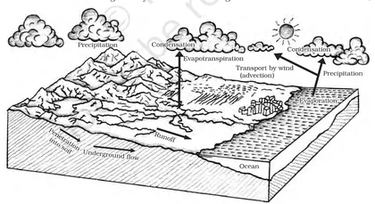
Introduction: This chapter, "Water (Oceans)", examines the world oceans as a dynamic physical system — their extent, structure, physical properties, movements and their interaction with the atmosphere and lithosphere. It introduces the major ocean basins, sea-floor relief, deposits and the processes that shape oceanic features. Importance: Oceans cover about 71% of Earth's surface and play a central role in climate regulation, the hydrological cycle, marine biodiversity, navigation, and as a source of natural resources. Understanding oceanic processes is essential for interpreting weather and climate patterns, coastal hazards, and human impacts such as pollution and resource exploitation. Key themes: The chapter focuses on (a) distribution and classification of oceans and seas; (b) ocean basin relief — continental shelf, slope, rise, abyssal plains, mid-ocean ridges and trenches; (c) physical properties of sea water — temperature, salinity and density and vertical variation; (d) movements of ocean water — waves, tides and currents (surface and deep); (e) ocean deposits and marine resources; and (f) the role of oceans in climate and human life, including conservation issues. What…
Learning Objectives
- Define oceans and state their global distribution, extent and interconnections
- Describe the major relief features of the ocean floor (continental shelf, slope, rise, abyssal plain, mid-ocean ridge, trench) with examples
- Draw and label a vertical bathymetric profile showing the continental shelf, slope, rise and deep-sea features
- Explain the causes, types and characteristics of ocean waves and their effects on coastal landforms
- Distinguish between tides and waves and explain the mechanism, types and regularity of tides
- Explain the origin, classification and global patterns of surface and deep ocean currents with illustrative examples (e.g., Gulf Stream, Humboldt Current)
- Analyze the concept of thermohaline circulation and explain its role in global heat transport and climate regulation
- Describe variations of seawater temperature and salinity with depth and latitude and explain their influence on water density and marine life distribution
Topics in this chapter
18 topics · tap a topic title to jump straight to it.
Introduction and Distribution of Oceans
What is an ocean? An ocean is a vast body of saline water that covers the major part of Earth’s surface and is divided into several principal basins. Oceans are larger and deeper than seas and connect with one another to form a continuous World Ocean.
Importance
- Climate regulation (heat transport via currents such as the Gulf Stream, influence on monsoons through ocean–atmosphere interactions).
- Source of food and livelihoods (fisheries, coastal economies).
- Transport and trade routes (shipping lanes, canals).
- Biological diversity and resources (marine ecosystems, minerals, energy).
Global distribution (basic facts)
- Oceans cover about 71% of Earth’s surface (≈ 361 million km²).
- They contain roughly 97% of Earth’s water and have an estimated volume of ~1.33 billion km³.
- Mean ocean depth ≈ 3,700 m; deepest point is the Mariana Trench (≈ 11,000 m).
The Five Principal Oceans (approximate characteristics)
- Pacific Ocean — largest and deepest; stretches from Americas to Asia/Australia. Key features: Ring of Fire (volcanic belts), deep trenches (Mariana Trench). Area ~165 million km².
- Atlantic Ocean — second largest, elongated N–S between Americas and Europe/Africa. Key features: extensive mid-Atlantic Ridge, important currents like the Gulf Stream. Area ~106 million km².
- Indian Ocean — lies mainly in the Southern Hemisphere between Africa, Asia and Australia; strongly influences South Asian monsoon. Area ~70 million km².
- Southern (Antarctic) Ocean — encircles Antarctica; characterized by strong circumpolar currents (Antarctic Circumpolar Current) and cold water masses. Area ~20 million km² (approx.).
- Arctic Ocean — smallest and shallowest, mostly within the Arctic Circle; covered seasonally by sea ice and influenced by continental runoff and ice melt. Area ~14 million km² (approx.).
How oceans are distributed and why
- Plate tectonics and continental arrangement: Positions of continents create ocean basins. Mid-ocean ridges (divergent boundaries) form new seafloor; trenches (convergent boundaries) consume it.
- Ocean basins and marginal seas: Major ocean basins are subdivided into seas, gulfs and bays by continental shapes (e.g., Mediterranean Sea, Arabian Sea).
- Bathymetric features: continental shelf, continental slope, continental rise, abyssal plain, mid-ocean ridge and trenches define depth and shape of each ocean basin.
- Climatic and oceanographic processes: winds, currents, temperature and salinity patterns further differentiate ocean regions (e.g., warm equatorial waters, polar water masses).
Boundaries and human links
- Natural boundaries between oceans are largely conventional (geographical lines and continental margins). For example, the line between Atlantic and Indian Oceans is commonly drawn from Cape Agulhas (South Africa) eastward.
- Human-made canals (Panama Canal, Suez Canal) link ocean basins and shorten trade routes, illustrating practical connectivity among oceans.
Key statistics (rounded)
- Total ocean area: ≈ 361 million km² (≈ 71% of Earth’s surface).
- Ocean volume: ≈ 1.33 billion km³.
- Mean depth: ≈ 3,700 m; deepest point ≈ 11,000 m (Mariana Trench).
- Average salinity: about 35 PSU (practical salinity units).
Summary: Oceans form a continuous global water body divided conventionally into five principal oceans. Their distribution is controlled by plate tectonics and continental positions, and their physical and climatic roles are central to Earth systems and human activities.
- Pacific Ring of Fire: the Pacific Ocean margins have many active volcanoes and earthquakes due to subduction zones and plate boundaries.
- Mariana Trench (Pacific): the deepest known part of the world’s oceans (~11,000 m), demonstrating how plate convergence forms deep trenches.
- Gulf Stream (Atlantic): a major warm ocean current that transports heat from the tropics to the North Atlantic, influencing climate in Western Europe.
- Indian Ocean and South Asian Monsoon: sea-surface temperature and pressure changes over the Indian Ocean help trigger and modulate the summer monsoon.
- Panama and Suez Canals: human-made links that connect the Pacific with the Atlantic and the Mediterranean/Indian Ocean, showing how oceans facilitate global trade.
- Percentage of Earth’s surface covered by an ocean or water body: (Area of ocean / Total surface area of Earth) × 100. Example: (361 million km² / 510 million km²) × 100 ≈ 71%.
- Mean depth of an ocean basin: Mean depth = Volume of ocean / Area of ocean. (Use consistent units, e.g., km³/km² → km → convert to m.)
- Hydrostatic pressure with depth: P = P0 + ρ g h, where P0 = atmospheric pressure (~101,325 Pa), ρ = density of seawater (~1025 kg/m³), g ≈ 9.8 m/s², h = depth (m). Example: at 1,000 m, additional pressure ≈ 1025×9.8×1000 ≈ 10.05×10^6 Pa (~99 atm), so total ≈ 100 atm.
- Fraction of Earth’s water in oceans: % = (Volume of ocean water / Total volume of Earth’s water) × 100. (Oceans hold ≈ 97% of Earth's water.)
Origin and Evolution of Ocean Basins
Summary: Ocean basins are formed and modified by plate-tectonic processes: continental rifting creates new oceanic crust at mid-ocean ridges (seafloor spreading), and old ocean crust is recycled at subduction zones (trenches). The plate-tectonics theory (a synthesis of Wegener’s continental drift, seafloor spreading, and mantle convection) explains the origin, configuration and evolution of oceans.
Key processes:
- Rifting and continental breakup: Mantle upwelling and crustal stretching cause a continental rift (example: East African Rift). Continued extension leads to a linear sea (example: Red Sea) and then a young ocean basin as oceanic crust forms.
- Seafloor spreading: New basaltic oceanic crust is produced at mid-ocean ridges (e.g., Mid-Atlantic Ridge, East Pacific Rise). The ridge is a site of high heat flow, shallow topography and symmetrical magnetic anomaly stripes recorded in the crust.
- Subduction and recycling: Oceanic lithosphere cools, becomes dense and is consumed at trenches (e.g., Mariana Trench). Subduction creates volcanic arcs, deep earthquakes and ultimately closes ocean basins.
- Mantle dynamics: Mantle convection, plume (hotspot) upwelling, ridge-push and slab-pull forces drive plate motions and therefore basin evolution.
Stages in the life of an ocean basin:
- Initial rift — continental crust stretches and faults (e.g., parts of East Africa).
- Linear sea — seawater floods the rift (e.g., early Red Sea).
- Young ocean — active mid-ocean ridge creates new oceanic crust; narrow ocean with high heat flow.
- Mature ocean — wide ocean basin with well-developed passive continental margins (e.g., Atlantic).
- Old ocean / closing ocean — subduction around margins consumes ocean floor and may lead to closure and continental collision (e.g., closing of the Tethys -> Himalaya).
Evidence for origin and evolution:
- Magnetic anomaly stripes: symmetric alternating polarity patterns on both sides of ridges (Vine–Matthews–Morley hypothesis).
- Age distribution of ocean floor: youngest at ridges, older away from ridges (seafloor age maps).
- Heat flow and shallow bathymetry at ridges; deep trenches at subduction zones.
- Ophiolites: fragments of oceanic crust emplaced on continents (e.g., Oman Semail ophiolite, Troodos in Cyprus) give direct samples of oceanic lithosphere.
- Earthquake distribution: shallow under ridges and deep in subduction zones.
Sedimentation and morphology: Sediment thickness increases toward continental margins and in older ocean basins. Abyssal plains are formed where fine sediments blanket older basaltic crust. Oceanic crust is thinner and denser than continental crust, leading to characteristic continental margins (passive vs active).
Practical implications: Understanding basin evolution explains distribution of marine resources (hydrocarbons on passive margins), earthquake/tsunami hazards at subduction zones, and the changing positions of continents and climates through geological time.
- Mid-Atlantic Ridge — slow spreading (~2–3 cm/yr) that opened the Atlantic after the breakup of Pangaea (~180 Ma); symmetric magnetic stripes record reversals.
- East Pacific Rise — fast-spreading ridge (up to ~15 cm/yr) with smoother topography and narrower ridge crest.
- Red Sea — example of an active continental rift transitioning into a narrow ocean (young ocean basin).
- Mariana Trench — deepest oceanic trench formed by subduction (old Pacific lithosphere subducting beneath an arc).
- Oman Semail Ophiolite and Troodos Ophiolite (Cyprus) — pieces of ancient oceanic crust uplifted onto land, providing direct evidence of oceanic lithosphere composition.
- Closure of the Tethys Ocean leading to the Himalayan orogeny — example of ocean basin closure by collision (suture zone).
- Seafloor spreading rate: V = d / t (V = velocity, d = distance of crust from ridge, t = age). Units: e.g., cm/yr or km/Ma. Conversion: 1 cm/yr = 10 km/Ma.
- Age from distance: t = d / V (rearrangement of the above). Useful for dating magnetic stripes: t (Ma) = distance (km) / V (km/Ma).
- Depth–age (empirical) relation for oceanic lithosphere: d(t) ≈ d0 + k · √t. A common approximation: d (m) ≈ 2500 + 350 × √(age in Ma). (Shows that ocean depth increases with the square root of crustal age due to cooling/subsidence.)
- Magnetic stripe method (practical use): spreading rate = (distance between two matching reversal isochrons) / (time between those reversals).
Relief of the Ocean Floor
Definition: The relief of the ocean floor (bathymetry) describes the shape, features and variations of the seafloor — from shallow continental shelves to the deepest ocean trenches. These features result from plate tectonics, volcanic activity, sedimentation and erosional processes.
Main zones and features:
- Continental Margin – the zone bordering continents and made of three parts:
- Continental shelf: gently sloping, extends from the shore to ~200 m depth (resource-rich, e.g., Bay of Bengal shelf, Grand Banks).
- Shelf break: where slope steepens, usually near 100–200 m depth.
- Continental slope: steep descent (hundreds to thousands of metres); often cut by submarine canyons (e.g., Monterey Canyon).
- Continental rise: an apron of sediments at base of slope formed by turbidity currents and deposition (e.g., Bengal Fan – world’s largest submarine fan).
- Deep-ocean Basin – beyond the continental margin:
- Abyssal plains: very flat, sediment-covered areas at ~3,000–6,000 m depth.
- Seamounts and guyots: submarine volcanoes (seamounts) and flattened extinct volcanoes (guyots); e.g., Hawaiian-Emperor seamount chain.
- Mid-ocean ridges: underwater mountain chains formed by seafloor spreading (e.g., Mid-Atlantic Ridge), often with central rift valleys and hydrothermal vents.
- Ocean trenches: very deep, narrow troughs formed at subduction zones (e.g., Mariana Trench — Challenger Deep ≈ 10,994 m).
Processes forming seafloor relief: Plate tectonics (seafloor spreading, subduction), volcanism (ridge volcanism, hot spots producing seamounts/islands), sedimentation (building continental rise & abyssal plains), erosion (submarine canyons) and isostasy.
Typical depth ranges (approx.): continental shelf: 0–200 m; slope: 200–3,000 m; rise: 3,000–4,000 m; abyssal plain: 3,000–6,000 m; trenches: down to >10,000 m.
Practical importance: Bathymetry guides navigation, fisheries, resource exploration (oil, gas, minerals), submarine cable routing, and helps understand earthquake/tsunami sources and marine ecosystems (hydrothermal vents, continental shelves).
Observing and mapping methods: echo-sounding (single-beam, multibeam), satellite altimetry (gravity anomalies), submersibles and seismic reflection for sub-surface layers.
- Mariana Trench (Pacific) — deepest known point; Challenger Deep ≈ 10,994 m.
- Mid-Atlantic Ridge — a divergent plate boundary forming an underwater mountain chain.
- Bengal Fan — largest submarine fan (thick sediment accumulation forming continental rise).
- Grand Banks (North Atlantic) — wide, productive continental shelf famous for fisheries.
- Monterey Submarine Canyon (California) — example of a deep submarine canyon cutting the continental slope.
- Hydrostatic pressure with depth: P = ρ g h (ρ ≈ 1025 kg·m⁻³ for seawater, g ≈ 9.81 m·s⁻²). Example: at 1,000 m, P ≈ 10.06 MPa (~100 atm).
- Depth from echo-sounding: depth = (v × t) / 2 (v ≈ 1500 m·s⁻¹ is average speed of sound in seawater; t is round-trip travel time).
- Slope (gradient) of seafloor: slope = vertical change / horizontal distance. Often expressed as tan(θ) = rise/run or percent slope = (rise/run)×100.
Ocean Deposits and Sediments
Overview
Ocean deposits and sediments are particles that settle and accumulate on the ocean floor. They record earth processes (weathering, erosion, biological production, chemical precipitation, cosmic input) and are classified by origin, grain size and depositional environment. Sediments control seafloor morphology, host mineral resources and serve as climate and environmental archives.
Major types by origin
- Terrigenous (Lithogenous) – derived from continental rock by rivers, waves, wind and glaciers. Common on continental shelves and near river mouths (e.g., sands and muds of the Bengal shelf).
- Biogenous – remains of marine organisms. Calcareous oozes (foraminifera, coccoliths) and siliceous oozes (diatoms, radiolaria). Found in areas of high productivity or specific depth ranges.
- Hydrogenous (Authigenic) – chemical precipitates from seawater: manganese nodules, ferromanganese crusts, phosphorites, evaporites.
- Cosmogenous – from space: micrometeorites and tektites; usually minor but globally distributed.
Depositional environments and typical deposits
- Continental shelf (neritic deposits) – coarse sands and silts, well-sorted terrigenous material; high-energy environment. Examples: wide sandy shelves with beach sands.
- Continental slope and rise – turbidity currents transport sands and produce turbidite sequences (graded beds). Continental rise accumulates submarine-fan deposits (e.g., Bengal Fan).
- Abyssal plains – fine clays and pelagic oozes (slow deposition rates), often very uniform and extensive.
- Mid-ocean ridges and hydrothermal zones – hydrothermal precipitates (sulfide deposits) near vents.
- Restricted basins and margins – chemical deposits like evaporites and phosphorites where evaporation or upwelling is intense.
Processes controlling sedimentation
- Supply – rivers, coastal erosion, glaciers, biogenic productivity, atmospheric dust.
- Transport – currents, waves, tides, turbidity currents, ice-rafting.
- Sorting and grain size – energy of environment sorts grains; high-energy = coarse, well-sorted; low-energy = fine, poorly sorted.
- Diagenesis – chemical alteration after deposition (compaction, cementation, authigenic mineral formation).
Importance
Ocean sediments are important for: reconstructing past climates (foraminifera and isotopes), locating mineral resources (manganese nodules, phosphorite, polymetallic sulfides), understanding sedimentary processes (turbidites as hydrocarbon reservoirs) and coastal management.
Simple classification by grain size (Wentworth, simplified): boulder > cobble > pebble > sand > silt > clay. Size indicates transport energy and depositional environment.
- Bengal Fan — the world's largest submarine fan formed by sediments from the Ganges–Brahmaputra system (terrigenous turbidite deposits on the continental rise).
- Clarion–Clipperton Zone (central Pacific) — extensive polymetallic manganese nodule fields (hydrogenous/authigenic nodules containing Mn, Ni, Cu, Co).
- Red Sea and Persian Gulf — modern examples of evaporite formation (halite and gypsum) in restricted basins.
- Southern Ocean and Antarctic margins — large deposits of diatomaceous (siliceous) ooze from high biological productivity.
- Monterey Canyon (California) — active turbidity currents producing turbidite sequences on the continental slope.
- Stokes' law for settling velocity of small spherical particles (laminar flow): v = (2/9) * ((ρ_p - ρ_f) * g * r^2) / μ — where v is settling velocity, ρ_p particle density, ρ_f fluid density, g gravity, r particle radius, μ dynamic viscosity. Useful to estimate how fast grains of different sizes settle.
- Sedimentation rate (average): R = Δthickness / Δtime — e.g., mm per thousand years (mm/ka) or cm/ky. Determined from dated cores.
- Mass accumulation rate (MAR): MAR = ρ_bulk * R — where ρ_bulk is bulk density of the sediment and R is thickness accumulation rate. Gives mass deposited per unit area per time.
Temperature of Ocean Waters
Definition: Temperature of ocean waters is a measure of the average kinetic energy of seawater molecules. It varies horizontally (with latitude, currents, coastal zones) and vertically (from warm surface layers to cold deep waters).
Main controls on ocean temperature
- Solar radiation and latitude: Incoming solar energy is strongest near the equator and weakest at poles. Angle of incidence and day length control seasonal and latitudinal differences.
- Atmospheric conditions: Cloud cover, air temperature, humidity and precipitation affect surface heating and cooling.
- Ocean currents: Warm currents (e.g., Gulf Stream, Kuroshio) transport heat poleward; cold currents (e.g., Humboldt, Canary) cool adjacent coasts.
- Vertical mixing and wind: Wind-driven turbulence and storms mix the surface layer, changing its temperature; mixing depth (mixed layer) varies by season and location.
- Upwelling and downwelling: Upwelling brings cold, nutrient-rich deep water to the surface (cooling the surface); downwelling pushes warm surface waters downward.
- Depth and light penetration: Solar radiation penetrates the upper ocean (visible light to ~100-200 m depending on clarity); below this the water is cold and stable.
- Salinity and density: Temperature and salinity together determine seawater density; colder and saltier water is denser, which influences vertical structure and circulation.
- Specific heat: Seawater has a high specific heat, so it warms and cools slowly, moderating climate.
Vertical temperature structure
- Mixed layer: Uppermost layer (typically 0–50/200 m) with nearly uniform temperature because of wind and wave mixing.
- Thermocline: Layer of rapid temperature decrease with depth (often between mixed layer and deep ocean). The thermocline is strong in the tropics, seasonal in mid-latitudes, weak or absent at high latitudes.
- Deep layer: Below the thermocline; temperature is low (about 0–4°C) and changes very slowly with depth.
Spatial and temporal patterns
- Surface temperatures: roughly 25–30°C in tropical seas, 5–20°C in mid-latitudes (seasonal), ~0–2°C in polar oceans where sea ice forms.
- Seasonal change: strongest in mid-latitudes (summer-warm surface, winter-cooling and deeper mixing), weakest in tropics and polar regions.
- Long-term change: ocean heat content is increasing with global warming, with consequences for sea level (thermal expansion) and climate systems (e.g., stronger storms, altered currents).
Why it matters
- Determines marine ecosystems (e.g., coral reefs require stable warm surface temperatures).
- Drives density differences that power thermohaline circulation (global conveyor belt).
- Controls weather and climate (heat storage and release affect monsoons, storms, and regional climates).
- Gulf Stream: A warm western boundary current that transports heat from the tropics to the North Atlantic, moderating winter climate in Western Europe.
- Humboldt (Peru) Current: A cold eastern boundary current that causes coastal upwelling off Peru, bringing cold, nutrient-rich water that supports one of the world’s richest fisheries.
- El Niño: Periodic warming of eastern tropical Pacific surface waters that disrupts global weather patterns, reduces upwelling off South America, and affects fisheries and rainfall worldwide.
- Seasonal thermocline in temperate seas: In summer the surface layer warms and a strong thermocline forms; in winter the surface cools and deep mixed layers develop.
- Coral bleaching: When sea surface temperature rises by about 1–2°C above the normal seasonal maximum, corals expel symbiotic algae and bleach, often leading to mortality.
- Heat required to change water temperature: Q = m · c · ΔT, where Q is heat (J), m is mass (kg), c is specific heat (~3850 J·kg⁻¹·K⁻¹ for seawater), and ΔT is temperature change (°C or K).
- Approximate radiative input per unit area at top of atmosphere: S_avg = S0 / 4 (S0 ≈ 1361 W·m⁻²), so S_avg ≈ 340 W·m⁻² (note: actual absorbed by ocean depends on albedo and atmospheric effects).
- Simple linearized density relation: ρ ≈ ρ0 [1 - α (T - T0) + β (S - S0)], where α is thermal expansion coefficient (~1–3 × 10⁻⁴ °C⁻¹), β is haline contraction coefficient (~7.6 × 10⁻⁴ per psu), T temperature, S salinity.
- Steric sea-level change from warming (approx.): Δh ≈ α · ΔT · H, where α is thermal expansion coefficient, ΔT is mean temperature change of layer, and H is layer thickness.
- Newton’s law of cooling (surface exchange approximation): q = h · (T_surface - T_air), where q is heat flux (W·m⁻²) and h is heat transfer coefficient (depends on wind, stability).
Salinity of Ocean Waters
Definition: Salinity is the total amount of dissolved inorganic salts in seawater, usually expressed as parts per thousand (‰, also called ppt) or in Practical Salinity Units (PSU). Average open-ocean salinity is about 35‰ (35 PSU).
Composition: Dissolved salts are dominated by a few major ions. Approximate percentage by mass of major ions: chloride ~55.0%, sodium ~30.6%, sulfate ~7.7%, magnesium ~3.7%, calcium ~1.2%, potassium ~1.1%. These proportions are nearly constant (the principle of constant proportions), so salinity can be estimated from any one major ion (commonly chloride).
How salinity is expressed and measured: Classic units: parts per thousand (‰) = grams of salts per kilogram of seawater (g kg−1). Modern oceanography uses Practical Salinity Scale (PSS-78), reported as PSU (unitless but numerically similar to ‰). Instruments: conductivity-temperature-depth (CTD) probes measure conductivity (related to salinity), temperature and pressure; water samples can be analyzed by titration for chlorinity.
Factors controlling salinity (surface and large-scale):
- Evaporation and precipitation: Evaporation removes fresh water and raises salinity; precipitation dilutes and lowers salinity. Subtropical belts (high evaporation) are saltier; regions with heavy rainfall are fresher.
- River inflow and runoff: River discharge supplies fresh water and reduces coastal salinity (e.g., Amazon, Ganges-Brahmaputra).
- Sea-ice formation and melting: Freezing expels salt and increases nearby salinity; melting adds fresh water and lowers salinity.
- Ocean mixing and currents: Surface currents, upwelling, and vertical mixing spread salinity horizontally and vertically; haloclines (strong salinity gradients) can form where mixing is weak.
- Temperature: Temperature modulates density and evaporation; warm surface waters evaporate more, often increasing salinity in subtropical gyres.
- Geographic basin effects: Restricted seas (Mediterranean, Red Sea) may have higher salinities due to high evaporation and limited exchange with open ocean.
Spatial patterns (typical): Surface salinity is highest in the subtropics (around 25°–35° N and S) where evaporation > precipitation (values ~36–38 PSU). Low salinity occurs near the equator (heavy rainfall and river inputs) and at high latitudes (ice melt and precipitation) — values can be <34 PSU or much lower in semi-enclosed seas and estuaries.
Vertical structure: Near the surface a mixed layer is maintained by wind and waves; below it a halocline is a zone of rapid salinity change with depth. In many open-ocean regions the deep ocean has nearly uniform salinity due to sluggish but large-scale circulation.
Role of salinity: Salinity, together with temperature and pressure, controls seawater density and thus stratification and ocean circulation. Higher salinity increases density. Salinity also affects sound speed, marine life, and chemical processes.
Human influences: Large-scale damming (reduces riverine inputs to coasts), freshwater consumption, and desalination plants (discharge of brine) can locally alter salinity. Climate change altering precipitation, evaporation patterns, and ice melt is shifting salinity distributions.
Measurement note: Because absolute salinity is conserved under mixing (to first order), salinity behaves as a conservative tracer for many oceanographic processes.
- Average ocean salinity: ≈35‰ (35 PSU).
- Mediterranean Sea: higher surface salinity, typically ≈37–39 PSU due to high evaporation and restricted exchange with the Atlantic.
- Red Sea: very high salinity (≈40 PSU or more) from intense evaporation in a narrow basin.
- Baltic Sea: very low salinity (≈5–10 PSU in many parts) because it is a semi-enclosed sea with large river input and limited ocean exchange.
- Amazon River mouth: large freshwater plume reduces surface salinity locally near the equator, producing strong horizontal salinity gradients.
- Dead Sea (inland salt lake): extreme salinity (~337‰) — an example of an isolated basin where salts concentrate dramatically.
- Salinity (ppt or ‰) = (mass of dissolved salts in grams / mass of seawater in kilograms) × 1000. Example: 35‰ means 35 g salts per 1 kg seawater.
- Mixing (conservative tracer): S_mix = (S1·V1 + S2·V2) / (V1 + V2), where Si and Vi are salinity and volume of two water parcels.
- Conservation during volume change (salt conserved): S_final = S_initial · (V_initial / V_final). For small fractional volume changes ΔV/V, ΔS/S ≈ −ΔV/V (useful to relate evaporation/precipitation to salinity change).
- Approximate density sensitivity: at typical ocean conditions, an increase of 1 PSU raises seawater density by roughly 0.7–0.8 kg·m−3 (value depends on temperature and pressure).
Density and Stratification of Seawater
What is density? Density (ρ) of seawater is mass per unit volume (ρ = m/V). Typical seawater density at the surface ranges about 1020–1030 kg·m−3, higher than fresh water (1000 kg·m−3).
What controls seawater density? Density is a function of salinity (S), temperature (T) and pressure (p): ρ = ρ(S, T, p).
- Salinity: higher salinity increases density because dissolved salts add mass.
- Temperature: increasing temperature decreases density (warmer water is lighter).
- Pressure: increasing pressure (with depth) slightly increases density by compressing water.
Stratification of the ocean occurs when layers of different density form one above the other. Because density generally increases downward, seawater tends to organize in vertical layers that resist vertical mixing. Key layers:
- Mixed layer (surface): The top layer (from surface to the mixed-layer depth, often 0–50(–100) m) is well mixed by wind and waves and is relatively uniform in T and S.
- Pycnocline: The layer of rapidly changing density with depth. Pycnocline is produced by the thermocline (rapid change in temperature) and/or halocline (rapid change in salinity). The pycnocline is the main barrier to vertical exchange of water, heat and nutrients.
- Deep layer: Below the pycnocline, density changes slowly with depth and waters are cold, salty and more homogeneous (the deep ocean).
Why stratification matters
- It controls mixing of heat, gases (like oxygen and CO2) and nutrients and therefore affects marine life and productivity.
- Strong stratification (strong pycnocline) suppresses upward nutrient fluxes, reducing surface productivity; weak stratification or mixing brings nutrients up and boosts productivity.
- Density-driven sinking at high latitudes (cold, salty water becomes dense and sinks) helps drive the global thermohaline circulation, an important component of climate regulation.
Spatial and temporal variations — Stratification varies with latitude (tropical oceans usually strongly stratified; polar oceans weakly stratified), season (winter mixed layer deepens due to cooling and storms; summer thermocline strengthens), and local processes (river input creates surface freshening and halocline; upwelling breaks stratification locally).
Stability — A stable water column has density increasing with depth. The strength of stratification is related to the vertical density gradient (dρ/dz); a larger gradient means stronger resistance to mixing.
- North Atlantic Deep Water formation: Cooling and increased salinity in high-latitude North Atlantic make surface water dense enough to sink, driving deep ocean circulation (thermohaline circulation).
- Estuaries: Freshwater input from rivers creates a low-salinity surface layer (halocline) over saltier seawater; this stratification controls pollutant dispersion and oxygenation.
- Monsoon-driven mixing in the Arabian Sea: Seasonal winds and storms deepen the mixed layer, breaking stratification and promoting phytoplankton blooms.
- Coastal upwelling (Peru/California): Wind-driven offshore transport of surface water allows nutrient-rich deeper water to rise where stratification is weak or locally disrupted, supporting fisheries.
- Seasonal thermocline in temperate seas: In summer a strong thermocline forms, isolating surface waters from deeper nutrient-rich waters; in winter cooling and storms destroy the thermocline and mix the water column.
- ρ = m / V (density = mass ÷ volume)
- ρ = ρ(S, T, p) (density is a function of salinity, temperature and pressure; precise values use oceanographic equations of state such as EOS‑80 or TEOS‑10)
- σ_t = ρ(S, T, 0) − 1000 (density anomaly or sigma‑t, commonly used in oceanography to compare densities)
- Qualitative partial derivatives: ∂ρ/∂S > 0 (density increases with salinity); ∂ρ/∂T < 0 (density decreases with temperature)
- Brunt–Väisälä frequency (stability indicator): N² = −(g/ρ) · (dρ/dz) (g = gravitational acceleration; positive N² indicates stable stratification)
Waves and Coastal Processes
Introduction: Waves are energy movements across the sea surface caused mainly by wind, but also by tides and seismic events (tsunamis). Coastal processes describe how waves, currents and tides shape shorelines by erosion, transportation and deposition of sediments.
Wave anatomy and motion:
- Crest: highest point; trough: lowest point.
- Wavelength (λ): horizontal distance between two successive crests or troughs.
- Wave height (H): vertical distance crest to trough; amplitude = H/2.
- Period (T): time between two successive crests passing a fixed point; frequency (f) = 1/T.
- Orbital motion: in deep water, water particles move in circular orbits that decrease rapidly with depth; in shallow water orbits become elliptical and are flattened at the bottom.
Types of waves:
- Wind waves: most common; created by wind energy transfer.
- Swell: long-travelled regular waves that form away from the wind source.
- Tidal waves: produced by gravitational pull of moon and sun (tides and tidal currents).
- Tsunamis: long-wavelength waves generated by underwater earthquakes, landslides or volcanic eruptions; behave as shallow-water waves in the open ocean.
Wave behaviour near coast:
- Shoaling: as waves enter shallower water, their wavelength shortens and height increases (energy concentrates), causing steepening.
- Breaking: when wave steepness (H/λ) exceeds a critical value (about 1/7) or when water depth becomes small relative to wave height, waves break forming surf and swash.
- Refraction: waves slow more in shallow water so crests bend to align with the shoreline, concentrating energy on headlands and dispersing it in bays.
- Diffraction: waves spread into sheltered zones behind obstacles or through gaps.
- Reflection: waves bounce off steep coasts or man-made structures.
Coastal processes:
- Erosion mechanisms: hydraulic action (pressure of water and air), abrasion/corrasion (sediment scours rock), attrition (sediments break down), solution (chemical dissolution).
- Transportation: sediment moves as traction (rolling of large particles), saltation (bouncing), suspension (fine particles carried in water) and solution (dissolved load).
- Longshore drift: oblique wave approach causes zig-zag movement of sediment along the coast, driven by the longshore current.
- Deposition: occurs where wave energy drops—forming beaches, spits, bars, tombolos and barrier islands.
Coastal landforms produced by erosion: cliffs, wave-cut platforms, sea caves, arches, stacks and blowholes. By deposition: beaches, spits (e.g., Hook-like landforms), tombolos (a sand link joining island to mainland), barrier islands and lagoons.
Role of tides and currents: Tidal ranges and tidal currents shape estuaries, tidal flats and mangrove zones. Strong tidal currents can prevent deposition in some coasts; microtidal vs macrotidal coasts show different landforms.
Tsunami behaviour: very long wavelength (tens to hundreds of km) so they travel fast in deep water (behave as shallow-water waves) and slow down near shore, causing large height amplification and severe inundation (example: 2004 Indian Ocean tsunami).
Human interaction and management: coastal protection methods include hard engineering (seawalls, groynes, breakwaters) and soft engineering (beach nourishment, dune regeneration, mangrove restoration). Each method has trade-offs—groynes trap sediment locally but can starve down-drift beaches.
Importance for geography students: Understanding waves and coastal processes explains shoreline evolution, hazards (erosion, flooding, tsunamis), resource distribution (beaches, estuaries), and informs sustainable coastal management.
- Shoaling and breaking: Storm waves approaching a gently sloping beach become higher and break as plunging or spilling breakers producing surf (common on many sandy beaches worldwide).
- Wave refraction concentrating erosion on headlands: Headlands (rocky promontories) receive focused wave energy and form cliffs and sea stacks; nearby bays accumulate sediment to form beaches (classic pocket bay-headland contrast).
- Longshore drift forming spits: Sediment transported along coasts by longshore currents can produce spits extending across bay entrances (e.g., many temperate coasts have spits—Spurn Head in UK as a famous example).
- Tsunami amplification: The 2004 Indian Ocean earthquake generated tsunamis that traveled across the ocean as long-wavelength waves and caused catastrophic coastal inundation when they shoaled near shore.
- Tidal landforms: The Sundarbans (Ganges-Brahmaputra delta) are shaped by strong tidal action and sediment deposition, producing mudflats and mangrove forests.
- Wave frequency: f = 1 / T, where T is the wave period (seconds).
- Deep-water wave speed (phase speed, c): c = gT / (2π) or c = sqrt(gλ / (2π)), where g is gravitational acceleration (≈9.81 m/s²), T is period (s), λ is wavelength (m).
- Shallow-water wave speed: c = sqrt(gd), where d is water depth (m).
- Relationship between wavelength and period (deep water): λ = gT² / (2π).
- Wave steepness: S = H / λ; waves typically break when S ≈ 1/7 (critical steepness).
- Tsunami shallow-water approximation: c ≈ sqrt(gd) (explains high speed in deep ocean and slowing near shore).
Tides
What are tides? Tides are the periodic rise and fall of sea level at a place caused primarily by the gravitational interaction of the Earth with the Moon and the Sun and by the centrifugal force resulting from the Earth-Moon system's rotation. They produce regular high and low waters along coasts and in oceans.
Main cause (simple/equilibrium view): The Moon's gravity attracts ocean water toward the side of Earth facing the Moon, producing a bulge (high tide). On the opposite side, a second bulge forms because the Earth is pulled slightly more toward the Moon than the water on that far side (centrifugal effect viewed in the rotating frame). If the Sun, Moon and Earth align, their effects combine; if at right angles, they partially cancel.
Dynamic view: Real tides differ from the ideal symmetric bulges because oceans sit in basins of varying depth and shape, continents block flow, and the Coriolis force (due to Earth's rotation) deflects tidal currents. These factors create complex patterns including amphidromic systems (rotating tidal waves with near-zero tidal range at the center) and resonances that can amplify tides in particular bays.
Types of tides:
- Semidiurnal: Two high and two low tides of approximately equal height each lunar day (~12 h 25 min between successive high tides). Common on many Atlantic coasts.
- Diurnal: One high and one low tide each lunar day (common in some parts of the Gulf of Mexico, Alaska).
- Mixed: Two high and two low tides each lunar day but of unequal heights (common on many Pacific coasts).
Spring and neap tides: Spring tides occur at new and full moon when Sun and Moon align and tidal ranges are largest. Neap tides occur at first and third quarters of the Moon when the Sun and Moon are at right angles and tidal ranges are smallest. The spring–neap cycle repeats about every 14.77 days (half the synodic month).
Special phenomena:
- Tidal bore: A steep front of incoming tide that travels upriver in a narrow funnel-shaped estuary or river (examples: Qiantang River, Severn bore).
- Large tidal ranges: Some places, such as the Bay of Fundy, experience very large tidal ranges (up to ~16 m) because of basin resonance and funnel shape.
Factors affecting tidal range and pattern: relative positions of Sun and Moon, distance of Moon from Earth (perigee/apogee), coastal shape (bays, estuaries), depth of water, local bathymetry and resonance, and Coriolis deflection.
Importance of tides: navigation and scheduling of ports, intertidal ecology (feeding and breeding of many species), coastal erosion and sedimentation patterns, tidal energy generation (tidal barrages and turbines), and fisheries/harvesting in intertidal zones.
Summary: Tides are periodic sea-level changes driven mainly by lunar and solar gravity and modified by Earth’s rotation and ocean basin geometry. Their regularity (diurnal, semidiurnal or mixed) and fortnightly modulation (spring/neap) are central to coastal processes and human activities.
- Bay of Fundy (Canada): one of the highest tidal ranges in the world, up to about 16 m, caused by basin shape and resonance.
- Qiantang River (China): famous tidal bore called the Silver Dragon; the incoming tide forms a visible wave that travels upriver.
- Severn Bore (United Kingdom): a well-known tidal bore attracting surfers and spectators.
- La Rance Tidal Power Station (France) and Sihwa Lake Tidal Power (South Korea): examples of utilising tidal range for electricity generation.
- Gulf of Khambhat and Gulf of Kutch (India): areas with large tidal ranges and strong tidal currents affecting ports and navigation.
- Newton's law of gravitation (context): F = G * (M * m) / d^2, where G is the gravitational constant, M and m are masses and d is distance between centres.
- Approximate tidal (differential) acceleration at Earth’s surface due to an external body (moon or sun): a_t ≈ 2 * G * M * R_earth / d^3. This shows tidal effect falls off roughly as 1/d^3, unlike gravity which falls as 1/d^2.
- Ratio of lunar to solar tidal effect: (a_lunar / a_solar) = (M_moon / M_sun) * (d_sun / d_moon)^3 ≈ 2.18 (so lunar tidal force ≈ 2.2 times solar).
- Tidal range (practical): tidal range = height of high tide − height of low tide.
- Typical tidal periodicities: semidiurnal interval ≈ 12 h 25 min between successive high tides; spring–neap cycle ≈ 14.77 days (half synodic month).
Ocean Currents and Surface Circulation
What are ocean currents? Ocean currents are large‑scale horizontal movements of seawater driven mainly by wind, the rotation of the Earth, differences in water density, and the shape of ocean basins. Surface currents affect the upper 100 200 m of the ocean and are most influenced by wind and the Coriolis effect.
Main driving forces
- Wind and global wind belts: Trade winds, westerlies and polar easterlies drag the sea surface and set large belts of water in motion.
- Coriolis effect: Earths rotation deflects moving water to the right in the Northern Hemisphere and to the left in the Southern Hemisphere, shaping current direction.
- Pressure gradients and gradients of sea surface height: Differences in sea level and pressure create geostrophic flows where pressure gradient force is balanced by Coriolis force.
- Density differences: Temperature and salinity variations produce thermohaline circulation that drives deep currents.
Key processes and concepts
- Ekman transport and spiral: Wind forces the surface layer which transmits motion downward in a spiralling pattern because of friction and Coriolis force. The net transport in the Ekman layer is approximately 90 degrees to the right of the wind in the Northern Hemisphere and to the left in the Southern Hemisphere.
- Gyres: Wind patterns and Coriolis effect create large circular systems called subtropical and subpolar gyres. Subtropical gyres spin clockwise in the Northern Hemisphere and anticlockwise in the Southern Hemisphere.
- Western intensification: Western boundary currents (for example Gulf Stream, Kuroshio) are narrow, deep and fast because of the variation of the Coriolis parameter with latitude and the shape of ocean basins.
- Upwelling and downwelling: When surface water is moved away from a coast (for example by Ekman transport) deep, cold, nutrient‑rich water rises (upwelling) supporting rich fisheries. Downwelling occurs where surface water converges and sinks.
- Thermohaline circulation: Slow, global circulation driven by density differences due to temperature and salinity. Often called the global conveyor belt, it connects surface and deep currents and plays a major role in long‑term climate regulation.
Effects of surface currents
- Climate regulation: Warm currents (eg Gulf Stream) moderate coastal climates by transporting heat polewards. Cold currents cool adjacent land areas and can create arid coastal climates.
- Marine ecosystems: Upwelling zones are highly productive and support major fisheries. Currents transport nutrients, larvae and pollutants.
- Human activities: Shipping routes use favorable currents; fisheries depend on upwelling. Changes in currents (eg El Niño) impact agriculture, fisheries and weather worldwide.
Typical examples include the Gulf Stream and North Atlantic Drift warming Western Europe, the cold California Current cooling the US West Coast, the Benguela Current powering rich fisheries off southwest Africa, and the Pacific equatorial currents whose variation produces El Niño and La Niña events.
Study tips
- Learn locations and directions of major currents and which hemisphere gyres rotate in.
- Understand cause and effect: how wind + Coriolis => Ekman transport => upwelling/downwelling => biological productivity.
- Use maps with arrows and cross‑section schematics to visualise surface and deep flows.
- Gulf Stream and North Atlantic Drift: warm, fast western boundary currents that transport heat to northwestern Europe, moderating climate.
- California Current: a cold eastern boundary current that cools the west coast of the USA and supports upwelling and fisheries.
- Benguela Current: cold upwelling system off southwest Africa, one of the world s richest fishing grounds.
- Kuroshio Current: western Pacific warm current that affects East Asian climate and marine life.
- El Niño Southern Oscillation (ENSO): weakened Pacific trade winds and changes in equatorial currents cause warming of eastern Pacific, disrupting fisheries and monsoons.
- Coriolis parameter: f = 2 Ω sin φ , where Ω = 7.2921 × 10^-5 s^-1 and φ is latitude.
- Ekman transport (magnitude): M = τ / (ρ f) , where τ is wind stress (N m^-2), ρ is seawater density (~1025 kg m^-3), f is Coriolis parameter. Direction: 90° to the right of wind in Northern Hemisphere (left in Southern).
- Geostrophic balance (horizontal): f k × v = - (1/ρ) ∇p . In component form: f v = (1/ρ) ∂p/∂x and f u = - (1/ρ) ∂p/∂y , relating pressure gradients to currents.
- Rossby number (to check importance of Coriolis): Ro = U / (f L) , where U is characteristic speed and L is length scale. Ro << 1 means Coriolis dominates.
Deep Ocean Circulation and Thermohaline Circulation
Definition: Deep ocean circulation (also called thermohaline circulation when driven primarily by temperature and salinity differences) is the large-scale movement of seawater in the global ocean interior, driven by variations in water density. Density differences arise mainly from changes in temperature (thermal) and salinity (haline), hence the name thermohaline.
Why it matters: Thermohaline circulation redistributes heat, salt, oxygen and nutrients around the globe. It influences climate (e.g., moderating European temperatures), marine ecosystems (by supplying nutrients through upwelling), and the long‑term carbon cycle (by sequestering CO2 in deep waters).
Basic mechanism:
- Surface waters at high latitudes cool and/or become saltier (for example, by sea ice formation which leaves salt behind), increasing their density.
- Dense surface water sinks to form deep water masses (e.g., North Atlantic Deep Water, Antarctic Bottom Water).
- Sunk water flows along the ocean basins as deep currents. Over centuries to millennia it upwells elsewhere, completes the global ‘‘conveyor belt,’’ and returns to the surface where wind-driven and surface processes act on it.
Key features of the vertical structure:
- Surface layer (mixed layer): Wind mixing produces a relatively uniform temperature and salinity near the surface.
- Thermocline: A zone of rapid temperature decrease with depth; also often coincides with a pycnocline (rapid density change).
- Deep layer: Cold, relatively stable waters with slow circulation and low temperature gradients.
Water masses and formation sites: Distinct deep water masses form where surface waters become dense enough to sink. Important examples: North Atlantic Deep Water (NADW) formed in the subpolar North Atlantic; Antarctic Bottom Water (AABW) formed around Antarctica. These water masses retain characteristics (temperature, salinity) and travel long distances as they fill ocean basins.
Dynamics and controls: Density ρ of seawater is a function of temperature (T), salinity (S) and pressure (p). Colder and saltier water is denser. Vertical stability depends on how density changes with depth: strong increase in density with depth (positive density gradient) suppresses vertical mixing. Mixing (by eddies, tides and bottom friction) and topography also shape deep currents.
Global conveyor belt concept: The thermohaline circulation is often visualized as a single global conveyor belt: warm surface currents (e.g., Gulf Stream) transport heat poleward; cooling and sinking at high latitudes feed deep return flows that travel through the basins and gradually upwell in other regions. Complete turnover times are long—typically on the order of centuries to a thousand years for the whole global loop.
Role in climate change: Changes in freshwater input (melting ice, increased precipitation) or warming can reduce surface water density and slow deep-water formation. A slowdown of the Atlantic Meridional Overturning Circulation (AMOC) is a concern because it would alter regional climates, sea level patterns, and ocean ecosystems.
Observational signatures: Thermohaline circulation is detected and studied using temperature–salinity (T–S) profiles, oxygen and nutrient concentrations, tracer studies (e.g., chlorofluorocarbons, radiocarbon), and direct current measurements from moorings and floats (e.g., Argo).
- Gulf Stream / North Atlantic Drift: A surface part of the ocean conveyor that brings warm water to northwestern Europe, moderating climate.
- North Atlantic Deep Water (NADW) formation: Surface cooling and brine rejection in the subpolar North Atlantic produce dense water that sinks and flows southward at depth.
- Antarctic Bottom Water (AABW): Very cold, salty water formed near Antarctica sinks to great depths and spreads into world oceans, filling abyssal basins.
- Peruvian upwelling: Coastal upwelling driven by wind and surface divergence brings nutrient-rich deep waters to the surface, supporting rich fisheries (e.g., anchoveta); changes in deep circulation influence productivity.
- AMOC slowdown concern: Increased Greenland meltwater can freshen the North Atlantic surface, reducing sinking and potentially weakening the meridional overturning circulation, with implications for regional climate.
- Density definition: ρ = m / V (mass per unit volume; seawater density ~1020–1030 kg/m³ depending on T and S).
- Approximate linear equation of state for seawater (linearized): ρ = ρ₀ [1 − α (T − T₀) + β (S − S₀)], where α is the thermal expansion coefficient and β is the haline contraction coefficient.
- Buoyancy frequency (Brunt–Väisälä frequency) indicating vertical stability: N² = (g / ρ) (dρ / dz), where g is gravitational acceleration, ρ is density and dρ/dz is the vertical density gradient. Larger N² => stronger stratification.
- Salinity units: Practical Salinity Unit (PSU) ≈ g of salt per kg of seawater (dimensionless).
Oceanic Zones and Marine Ecosystems
Overview
Oceans are vertically and horizontally zoned by light, depth, distance from shore and bottom substrate. These zones determine physical conditions (light, temperature, pressure), biological communities and ecosystem functioning. Understanding oceanic zones helps explain where organisms live, how energy flows and how human impacts affect marine life.
Horizontal (Coastal to Open Ocean) Zones
- Supralittoral (Splash) Zone – above high tide, influenced mainly by spray, includes salt-tolerant lichens and crustaceans.
- Littoral / Intertidal Zone – between high and low tide; organisms tolerate immersion and exposure (e.g., barnacles, mussels, tidal pools).
- Neritic Zone (Continental Shelf) – from low tide mark to the edge of the continental shelf (typically to ~200 m). High nutrient input, productive fisheries, coral reefs and kelp forests occur here.
- Oceanic (Pelagic) Zone – open ocean beyond the shelf. Light and nutrients limit productivity; organisms are free-swimming or drifting (plankton, nekton).
Vertical / Depth-based (Pelagic) Zones
- Epipelagic (Euphotic / Sunlit) 0–~200 m – sufficient light for photosynthesis; highest primary productivity (phytoplankton).
- Mesopelagic (Twilight) ~200–1000 m – diminished light, many vertically migrating organisms; reduced primary production.
- Bathypelagic ~1000–4000 m – darkness, cold, high pressure; organisms rely on detrital rain or predation.
- Abyssopelagic ~4000–6000 m – near-bottom plains; sparse life adapted to extreme conditions.
- Hadal Zone >6000 m – deepest trenches (e.g., Mariana Trench); specialized fauna.
Benthic Zones (linked to depth and substrate): supralittoral, littoral, sublittoral (shelf), bathyal (slope), abyssal (plain), hadal (trenches). Benthic communities include sessile organisms (corals, sponges), burrowers and scavengers.
Key Environmental Gradients
- Light: Exponentially decreases with depth. Euphotic zone supports photosynthesis.
- Temperature: Surface warmed by sun; thermocline (sharp gradient) separates warm surface from cold deep water.
- Pressure: Increases ~1 atm every 10 m of depth; affects physiology and body structure of deep-sea life.
- Salinity: Varies with evaporation, precipitation, river input; influences water density and circulation.
- Nutrients & Oxygen: Nutrients often low at surface in open ocean (consumed by phytoplankton); higher at depth due to decomposition. Oxygen minimum zones occur in some mesopelagic layers.
Marine Ecosystems & Their Characteristics
- Coral Reefs – tropical, high biodiversity, built by calcium-carbonate secreting corals in shallow, clear, warm water. Symbiosis with zooxanthellae (algal symbionts) drives high productivity and calcification.
- Mangrove Forests – intertidal tropical trees that trap sediments, protect coasts, nurseries for fish (example: Sunderbans, India).
- Estuaries – river mouths with brackish water, high nutrient loads and productivity; important nursery grounds (e.g., the Ganges–Hooghly estuary).
- Pelagic Open-Ocean – dominated by planktonic food chains; low nutrients in many gyres but very large in area, so important for global carbon cycling.
- Benthic Communities – include kelp forests (temperate shelves), soft-sediment communities, deep-sea corals and hydrothermal vent communities (chemosynthetic primary production at vents such as those on the Galápagos Rift).
Productivity and Food Webs
Primary producers (phytoplankton, seaweeds, seagrasses) fix carbon. Gross Primary Production (GPP) minus respiration (R) gives Net Primary Production (NPP). Energy passes through trophic levels: phytoplankton → zooplankton → small fish → larger predators. Coastal and upwelling zones show the highest NPP; oligotrophic open ocean has low surface nutrients and low NPP.
Human Impacts and Conservation
Major threats: overfishing, habitat destruction (mangroves, coral reefs), pollution (plastics, oil), eutrophication, climate change (sea warming, coral bleaching), and ocean acidification (reduced carbonate availability for shells/corals). Conservation tools: marine protected areas (MPAs), sustainable fisheries, mangrove restoration, pollution control and international agreements (e.g., regulations on shipping and fisheries).
Summary
Oceanic zones define the physical setting and biological communities. From sunlit coastal reefs and productive upwelling regions to deep, dark trenches and chemosynthetic vent ecosystems, each zone hosts adapted life and contributes to global biogeochemical cycles. Protecting diverse marine ecosystems is essential for biodiversity, fisheries and climate regulation.
- Great Barrier Reef (Australia) — largest coral reef system showing zonation: reef crest, lagoon, and outer reef; biodiverse and vulnerable to bleaching.
- Sunderbans (India/Bangladesh) — extensive mangrove ecosystem, important coastal protection and fish nursery.
- Peruvian/Humboldt Upwelling (off Peru) — strong coastal upwelling driven by winds and the Humboldt Current, supports one of the world's richest fisheries.
- Mariana Trench (Pacific) — deepest hadal zone (~11,000 m) with uniquely adapted organisms and extreme pressure conditions.
- Hydrothermal vents (East Pacific Rise / Galápagos Rift) — deep-sea chemosynthetic ecosystems where bacteria use hydrogen sulfide to support diverse fauna (tube worms, clams).
- Monterey Bay (California) — example of a productive continental shelf/neritic ecosystem with seasonal upwelling and rich marine life.
- Hydrostatic pressure with depth: P = P0 + ρ g h ; where P is pressure at depth, P0 is surface atmospheric pressure (~101325 Pa), ρ is seawater density (~1025 kg/m³), g is acceleration due to gravity (~9.81 m/s²), h is depth (m).
- Light attenuation (Lambert–Beer law approximation): I(z) = I0 · e^(−kz) ; I(z) is irradiance at depth z, I0 is surface irradiance, k is the light attenuation coefficient (m⁻¹).
- Primary production relation: NPP = GPP − R ; where GPP is gross primary production and R is autotrophic respiration.
- Approximate seawater density influence: seawater density increases with salinity and decreases with temperature — used conceptually in circulation and stratification studies (no single simple universal algebraic expression).
Coral Reefs and Estuaries
Overview
Coral reefs and estuaries are two important coastal and nearshore marine environments with distinct physical, chemical and biological characteristics. Both provide critical ecosystem services — biodiversity, fisheries, coastal protection and nutrient cycling — but they form and function under different environmental regimes.
Coral Reefs
- Definition and types: Coral reefs are limestone structures formed by the skeletons of colonial cnidarians (scleractinian corals). Major reef types are fringing reefs, barrier reefs and atolls.
- Formation and biology: Reef-building corals host symbiotic algae (zooxanthellae) that perform photosynthesis and provide most of the coral's energy. Coral polyps secrete calcium carbonate (aragonite) to build skeletons; over long timescales these skeletons accumulate to form reef structures.
- Physical and chemical requirements: Warm sea-surface temperatures (approx. 20–30°C), clear shallow water (light penetration; optimal depth usually <25–30 m), normal marine salinity (~32–40‰), stable substrate, and low nutrient (oligotrophic) conditions favour reef growth.
- Reef zones: Reef crest, fore-reef (slope), reef flat and lagoon (where present). Each zone has distinct wave exposure, species composition and productivity.
- Ecological importance: High biodiversity (often called the 'rainforest of the sea'), nursery grounds for fish, shoreline protection by dissipating wave energy, and sources of sand and calcium carbonate.
- Threats: Coral bleaching (thermal stress causing loss of zooxanthellae), ocean acidification (reduced carbonate ion concentration reduces calcification), pollution and sedimentation, destructive fishing, coastal development and overfishing.
- Conservation: Marine Protected Areas (MPAs), reef restoration (coral gardening, transplanting), watershed management to reduce sediment and nutrient runoff, and global CO2 mitigation.
Estuaries
- Definition: Estuaries are semi-enclosed coastal bodies of water where freshwater from rivers mixes with seawater. They are dynamic transition zones between riverine and marine environments.
- Types by origin: Coastal plain (drowned river valley/ria), fjords (glacially carved), bar-built (sandbar separated), and tectonic estuaries.
- Mixing classes: Salt-wedge (strong stratification with a sharp salinity front), partially mixed, well-mixed (vertically uniform salinity), and fjord-type (strong stratification, deep basins).
- Characteristics: Brackish water (salinity gradient from fresh to marine), strong tidal influence, high sedimentation in some estuaries, and elevated nutrient concentrations due to river inputs and trapping of materials.
- Ecological importance: Highly productive (important nursery grounds for many fish and shellfish), provide habitat for birds and other wildlife, act as filters for pollutants and sediments, and are often centers of human settlement and commerce.
- Threats: Pollution (industrial and agricultural runoff), eutrophication leading to hypoxia, reduced freshwater inflow from damming, land reclamation, invasive species, and overdevelopment.
- Conservation: Integrated watershed and coastal zone management, protection of wetlands and mangroves, maintaining environmental flows, pollution control, and habitat restoration.
Connections and contrasts
Coral reefs thrive in clear, low-nutrient, high-light conditions and are sensitive to increases in sediment and nutrients. Estuaries are naturally nutrient-rich and turbid and support high primary productivity but are sensitive to altered freshwater regimes and pollution. Both are vulnerable to climate change — reefs to warming and acidification, estuaries to sea-level rise, altered river flows and changing salinity regimes.
Key processes to understand
- Calcification and carbonate chemistry in reefs (how carbonate ion concentration controls coral growth).
- Mixing and stratification in estuaries (how tides and river flow determine salinity profiles).
- Nutrient dynamics and primary productivity differences: low-nutrient reefs vs nutrient-rich estuaries.
Teaching tips / study focus for Class 11
Be able to: name reef types and reef zones, explain conditions required for reef growth, describe causes and consequences of coral bleaching and ocean acidification, classify estuaries by origin and mixing type, draw a salinity gradient for different estuary types, and list ecosystem services and major threats for both habitats.
- Great Barrier Reef (Australia) — the world's largest coral reef system, a classic example of diverse fringing, barrier reef and continental shelf-associated reef communities.
- Maldives and atolls — ring-shaped atolls formed atop subsiding volcanoes with lagoon ecosystems.
- Red Sea reefs — corals adapted to higher salinities and temperature ranges.
- Sundarbans (Ganges–Brahmaputra delta, India/Bangladesh) — a large mangrove-estuarine complex and nursery ground for fish, also demonstrating sediment trapping and tidal dynamics.
- Thames Estuary (UK) — example of a heavily modified, tidal estuary subject to navigation, urbanisation and water quality management.
- Chesapeake Bay (USA) — a large temperate estuary facing eutrophication and hypoxia from agricultural runoff.
- Salinity (simple mass fraction): Salinity (‰) = (mass of dissolved salts / mass of seawater) × 1000
- Conservative mixing of salinity in an estuary (mass-balance): S_mixed = (S_fresh × Q_fresh + S_sea × Q_sea) / (Q_fresh + Q_sea), where Q = volumetric flow.
- Tidal prism (estimate of exchanged water volume): Tidal Prism (Tp) = Area of estuary (A) × Mean tidal range (h).
- Light attenuation with depth (relevant for reef photosynthesis): I(z) = I0 × e^(−kz), where I0 = surface irradiance, k = light attenuation coefficient, z = depth.
- Aragonite saturation state (controls calcification): Ω_arag = [Ca2+][CO3^2−] / Ksp(arag). Lower Ω reduces coral calcification (conceptual; requires chemical speciation for numeric work).
Marine Resources and Economic Importance
What are marine resources? Marine resources are the biological and non-biological materials and services obtained from the oceans, seas, coasts and continental shelves. They include living resources (fish, plankton, seaweeds), non-living mineral and energy resources (petroleum, natural gas, sand, manganese nodules), and ecosystem services (coastal protection, climate regulation, tourism).
Classification (simple):
- Living (renewable): plankton, finfish, shellfish, seaweeds, coral reefs, mangroves.
- Non-living (mineral/energy): marine salt, sand and gravel, heavy minerals, polymetallic (manganese) nodules, hydrothermal sulfides, seabed minerals, crude oil and natural gas (offshore), methane hydrates.
- Renewable energy: tidal, wave, offshore wind, ocean thermal energy conversion (OTEC).
- Services: shipping, ports, tourism, coastal protection, carbon sequestration, biotechnology.
Legal and management context: Under UNCLOS (United Nations Convention on the Law of the Sea) coastal states have sovereign rights for exploration and use of natural resources within their Exclusive Economic Zone (EEZ) up to 200 nautical miles (nm) from the baseline. Territorial sea extends up to 12 nm. (1 nm = 1.852 km.)
Major economic roles:
- Fisheries and aquaculture: food security, employment, export earnings. Small-scale coastal fisheries are vital for livelihoods in many developing countries.
- Transport and trade: >80% of global trade by volume moves by sea. Major shipping lanes and chokepoints (e.g., Strait of Malacca, Suez Canal) are critical to international commerce.
- Energy: offshore oil and gas are major national revenues (e.g., Mumbai High). Growth in offshore wind farms and tidal projects supports energy diversification.
- Minerals: seabed mining (manganese nodules, polymetallic sulfides) has potential strategic value for copper, nickel, cobalt.
- Tourism and recreation: coastal and marine tourism (beaches, coral reefs, diving) generate income and jobs (e.g., Goa, Andaman & Nicobar Islands).
- Coastal protection and climate regulation: mangroves and coral reefs protect shorelines from erosion and storms and provide carbon sinks.
Environmental and sustainability issues: overfishing, habitat destruction (mangroves, coral reefs), marine pollution (plastics, oil spills), ocean acidification and warming. Sustainable management (regulated fishing, marine protected areas, pollution control, responsible offshore development) is essential to maintain long-term economic benefits.
Summary: Marine resources underpin food, energy, trade and livelihoods for billions. Their economic importance is huge, but sustainable governance is required to balance extraction with conservation to ensure continued benefits for present and future generations.
- India's Exclusive Economic Zone (EEZ) of about 200 nm provides rights to marine resources—India’s EEZ area ≈ 2.02 million sq. km (practical example of national marine resource jurisdiction).
- Mumbai High — major offshore oilfield supplying significant portion of India’s crude from the Arabian Sea (example of offshore hydrocarbons).
- Lakshadweep and Andaman & Nicobar Islands — coral reefs and tourism (example of marine biodiversity supporting ecotourism).
- Clarion–Clipperton Zone (central Pacific) — area rich in polymetallic (manganese) nodules, targeted for deep-sea mining exploration (example of seabed mineral interest).
- North Sea offshore wind farms (UK/Denmark) and South Korea’s Sihwa Lake Tidal Power Station — examples of marine renewable energy projects.
- Strait of Malacca and Suez Canal — critical shipping chokepoints that show the oceans’ role in global trade and geopolitics.
- Convert nautical miles to kilometres: distance_km = distance_nm × 1.852
- Area of a circular EEZ (approximation): Area = π × (R_km)^2, where R_km = 200 nm × 1.852 (useful for rough area estimation of a full 200 nm zone around a point).
- Catch per unit effort (CPUE) — fisheries productivity indicator: CPUE = Total catch / Effort (e.g., days of fishing, number of nets).
- Salinity (approx., in parts per thousand): Salinity (‰) = mass_of_dissolved_salts (g) / mass_of_seawater (kg). Typical open-ocean value ≈ 35‰.
- Basic density relation: density (ρ) = mass / volume. (Seawater density increases with salinity and decreases with temperature — used in oceanography and resource extraction planning.)
Sea Level Change and Coastal Management
What is sea level change? Sea level change is the variation in the average height of the ocean surface relative to the land. It can be measured globally (mean sea level) or locally (relative sea level). Changes may be short-term (tides, storm surge) or long-term (decadal to millennial trends).
Types and causes
- Eustatic change – a global change in ocean volume or mass (for example, melting of glaciers and ice sheets increases ocean mass; thermal expansion increases ocean volume).
- Isostatic (or relative) change – vertical movement of land (uplift or subsidence) that changes sea level relative to the coast (e.g., post-glacial rebound, tectonics, groundwater withdrawal causing subsidence).
- Steric change – change in sea level due to change in water density with temperature and salinity; thermal expansion (warmer water occupies more volume) is the main steric effect.
- Dynamic and meteorological effects – changes caused by ocean currents, winds, atmospheric pressure (e.g., El Niño, storm surges).
Contemporary trend: Satellite altimetry and tide-gauge records show a globally averaged sea level rise of about 3.0–3.5 mm per year in recent decades (IPCC and observational estimates), but rates vary regionally due to ocean circulation and land motion.
Impacts of rising sea level
- Inundation and permanent loss of low-lying land and islands.
- Increased coastal erosion and shoreline retreat.
- Saltwater intrusion into groundwater and agricultural soils.
- Loss of coastal habitats (mangroves, salt marshes) and biodiversity.
- Higher storm surge heights and more frequent flooding of infrastructure, settlements and roads.
- Socioeconomic consequences: displacement of communities, damage to ports, tourism and fisheries.
Coastal management approaches
- Hard engineering – physical structures built to reduce erosion or block waves: seawalls, breakwaters, groynes, revetments. Effective locally but expensive and can transfer erosion down-coast.
- Soft engineering – works with natural processes: beach nourishment, dune restoration, managed realignment (allowing some areas to flood to create wetlands), planting vegetation (mangroves, salt marshes).
- Ecosystem-based adaptation – restoring or conserving natural buffers such as mangroves and coral reefs which attenuate waves and reduce erosion while providing biodiversity benefits.
- Policy and planning – zoning (no-build setbacks), land-use planning, building codes, early warning systems, insurance, and community-based preparedness.
- Integrated Coastal Zone Management (ICZM) – holistic approach combining engineering, ecology, social and economic planning to achieve sustainable use and protection of coasts.
Principles for selecting management options: consider cost-effectiveness, environmental impact, longevity, flexibility (ability to adapt to accelerating sea level rise), equity (protecting vulnerable communities), and maintaining natural coastal dynamics where possible.
Class 11 relevance (how students should think about it): understand the physical mechanisms (thermal expansion, melting ice, land movement), be able to explain local vs global effects, list impacts on people and ecosystems, and describe a range of management measures with examples.
- The Netherlands: long history of large-scale engineering (dikes, Delta Works) to keep land below sea level habitable — an example of extensive hard engineering and national planning.
- Sundarbans (India–Bangladesh): mangrove loss, cyclones and sea-level rise increase inundation and erosion; restoration of mangroves and community shelters are part of adaptation.
- Maldives: a nation of low-lying atolls considering seawalls, land reclamation and international advocacy; example of extreme vulnerability of small island states.
- Bangladesh: embankments, cyclone shelters, early-warning systems and community-based adaptation demonstrate soft and social measures in a high-risk developing-country context.
- Venice (Italy) and the MOSE project: movable barriers to protect the lagoon from exceptional tides and storm surge; example of large-scale engineering with environmental trade-offs.
- Louisiana (USA): rapid land subsidence plus sea-level rise has caused extreme wetland loss and coastal retreat — highlights the combined effect of VLM and eustatic rise.
- Rate of sea level change: rate = (h2 - h1) / (t2 - t1) (units: e.g., mm yr⁻¹).
- Relative sea level change (RSL): RSL = Eustatic Sea Level change (ESL) + Vertical Land Motion (VLM). (If VLM is negative (subsidence), RSL increases.)
- Steric (thermal) expansion (volumetric, approximate): ΔV / V ≈ β · ΔT, where β is the volumetric thermal expansion coefficient and ΔT is temperature change.
- Time to inundation (simple estimate): time ≈ elevation_above_MSL / rate_of_rise. (Example: 1.0 m ÷ 3.3 mm yr⁻¹ ≈ 303 years.)
Oceanographic Methods and Tools
Oceanographic methods and tools are techniques and instruments used to study the physical, chemical, biological and geological properties of the oceans. Methods are broadly grouped into direct (in-situ) and indirect (remote) approaches. They enable mapping of seafloor bathymetry, measurement of temperature, salinity, currents, waves and sea level, sampling of sediments and organisms, and detection of sub-surface structures.
1. Direct (In‑situ) Methods
- Sounding and Bathymetry: Traditional lead‑line sounding was replaced by echo‑sounding. A pulse is emitted and depth is calculated from travel time. Modern systems: single‑beam echo sounders, multibeam echo sounders (detailed bathymetric maps), and side‑scan sonar (seafloor imagery).
- Profiling Instruments: CTD (Conductivity‑Temperature‑Depth) packages measure salinity (from conductivity), temperature and pressure vs depth. XBTs (expendable bathythermographs) measure temperature profiles. ARGO floats autonomously drift and profile temperature/salinity to 2000 m.
- Current Measurement: Mechanical current meters, acoustic Doppler current profilers (ADCPs) measure current speed and direction at many depths. Drogues/drift bottles track near‑surface flow.
- Sampling Tools: Grab samplers (surface sediments), corers (long sediment cores for stratigraphy and paleo‑climate), dredges, plankton nets and water bottles for chemical/biological samples.
- Submersibles and ROVs: Manned (e.g., Alvin) and unmanned remotely operated vehicles provide direct observation, sampling and high‑resolution imagery of the seabed and hydrothermal vents.
- Tide Gauges and Wave Buoys: Measure sea level, tidal changes and wave height. DART (Deep‑ocean Assessment and Reporting of Tsunamis) buoys detect tsunami waves.
2. Indirect (Remote) Methods
- Satellite Remote Sensing: Radar altimeters (TOPEX/Poseidon, Jason series) measure sea surface height (useful for currents and sea level rise). Passive sensors measure SST (sea surface temperature), ocean colour (chlorophyll) and surface winds; microwave and radar map surface roughness.
- Marine Seismic Surveys: Air‑gun sources and hydrophone arrays map sediment layers and tectonic structures beneath the seafloor using reflected seismic waves.
- Magnetometers and Gravimeters: Map magnetic and gravity anomalies related to seafloor structure and tectonics.
3. Uses and Integration
Combining shipboard tools, autonomous floats, buoys and satellites gives a comprehensive picture of ocean state — bathymetry for navigation and habitat mapping, CTD and ARGO data for climate monitoring, ADCP and satellite altimetry for current systems, seismic surveys for resource exploration and tectonic studies.
Practical considerations: instrument calibration, correction for sound speed changes with temperature/salinity/pressure, accurate GPS positioning for georeferencing, and synchronized time series for dynamic studies.
- Mapping the Mariana Trench and other deep‑sea features using multibeam echo sounders and shipboard navigation systems.
- Discovery and imaging of the RMS Titanic using side‑scan sonar and ROVs for close visual inspection.
- ARGO float network providing global temperature and salinity profiles to 2000 m, used in climate monitoring and seasonal forecasting.
- TOPEX/Poseidon and Jason satellites measuring sea surface height to monitor ocean currents and sea level rise.
- Use of CTD casts and sediment coring during International Ocean Discovery Program (IODP) cruises to reconstruct past climate from sediment layers.
- DART buoys and coastal tide gauges used in tsunami detection and early warning systems (e.g., Pacific Tsunami Warning System).
- Depth from echo sounder: d = (c × t) / 2, where d = depth, c = speed of sound in seawater (~1500 m/s, varies with T, S, P), and t = round‑trip travel time.
- Hydrostatic pressure: P = P0 + ρ g h, where P0 = atmospheric pressure, ρ = seawater density (~1025 kg/m³), g = 9.81 m/s², h = depth.
- Salinity from chlorinity (classical relation): S (‰) ≈ 1.80655 × Cl (‰).
- Coriolis parameter: f = 2 Ω sin φ (Ω = Earth’s rotation rate = 7.2921×10⁻⁵ s⁻¹, φ = latitude).
- Ekman transport (per unit width): M_E = τ / (ρ f), where τ = wind stress, ρ = seawater density, f = Coriolis parameter.
- Geostrophic approximation (balance of Coriolis and pressure gradient): f v_g = - (1/ρ) ∂p/∂x and f u_g = (1/ρ) ∂p/∂y. For sea surface slope η: v_g ≈ (g / f) (∂η/∂x).
Human Impacts, Pollution and Conservation
Overview
Human activities have profoundly changed the oceans through direct physical alteration, resource extraction and the release of wastes. These changes reduce biodiversity, alter ecosystem functioning and affect human well‑being. Conservation and management aim to reduce impacts, restore ecosystems and ensure sustainable use.
Human impacts on the marine environment
- Overfishing — removal of fish faster than populations can reproduce leads to stock collapse (e.g., Atlantic cod decline). It also causes bycatch (non‑target species mortality).
- Habitat destruction — coastal development, dredging, trawling and reclamation damage habitats such as coral reefs, seagrass beds and mangroves that provide nursery and feeding grounds.
- Resource extraction — oil and gas drilling, deep‑sea mining and sand mining disturb seabed and can release pollutants.
- Shipping and transport — ballast water transfers invasive species; shipping causes oil spills, noise pollution and collision risk to marine mammals.
Types of pollution and processes
- Plastic pollution — macroplastics and microplastics cause entanglement, ingestion and act as vectors for chemicals. Plastics accumulate in gyres (e.g., Great Pacific Garbage Patch).
- Oil pollution — spills coat organisms, reduce insulation of birds and cause long‑term toxic effects (e.g., Deepwater Horizon, 2010).
- Organic pollution and pathogens — untreated sewage increases biochemical oxygen demand (BOD), reduces dissolved oxygen and can cause harmful algal blooms.
- Nutrient pollution (eutrophication) — excess nitrogen and phosphorus from agriculture and sewage causes algal blooms, hypoxia and dead zones (e.g., Gulf of Mexico dead zone).
- Chemical pollution — heavy metals (mercury, lead), persistent organic pollutants (PCBs, DDT) bioaccumulate and biomagnify up food chains causing health impacts (e.g., Minamata mercury poisoning historically).
- Thermal and noise pollution — heated effluents and underwater noise (sonar, shipping) stress organisms and disrupt behaviour and breeding.
Impacts on ecosystems and people
- Loss of biodiversity, altered food webs and reduced fisheries yields.
- Coastal communities lose livelihoods, tourism and cultural values.
- Human health risks from contaminated seafood and polluted beaches.
Conservation and management measures
- Protected areas — Marine Protected Areas (MPAs) and no‑take zones protect habitats and allow stocks to recover; examples include the Great Barrier Reef Marine Park (zoned management).
- Sustainable fisheries — quotas, size limits, seasonal closures, gear restrictions, community co‑management and catch‑monitoring reduce overfishing and bycatch.
- Pollution control — wastewater treatment, stricter industrial discharge limits, agricultural best management practices (buffer strips, reduced fertilizer use) and bans on harmful chemicals.
- Plastic reduction and waste management — source reduction, recycling, extended producer responsibility and beach cleanups to cut marine plastic input.
- Habitat restoration — mangrove planting, coral restoration and seagrass rehabilitation improve coastal resilience and fisheries productivity.
- International agreements and regulation — MARPOL (marine pollution by ships), UNCLOS provisions, regional seas conventions and national coastal zone management policies.
- Monitoring, research and public awareness — regular monitoring of water quality, biological indicators and community education are vital for adaptive management.
Class 11 learning focus
Understand the causes, processes and consequences of human impacts on oceans; be able to relate local and global examples and identify practical conservation measures.
- Great Pacific Garbage Patch — accumulation zone of plastic debris in the North Pacific gyre caused by ocean currents and global plastic waste inputs.
- Deepwater Horizon oil spill (Gulf of Mexico, 2010) — large oil release with long‑term impacts on fisheries, wetlands and coastal wildlife.
- Gulf of Mexico dead zone — seasonal hypoxic area caused by nutrient runoff (mainly from Mississippi River agricultural fertilizers) leading to fish kills and altered ecosystems.
- Collapse of Atlantic cod fisheries (Northwest Atlantic) — overfishing in the late 20th century leading to stock collapse and socioeconomic impacts on coastal communities.
- Coral bleaching on the Great Barrier Reef — warming waters and pollution have caused wide‑scale loss of coral cover, affecting biodiversity and tourism.
- Mangrove loss and restoration (Sundarbans region) — conversion to aquaculture and coastal development reduced mangroves; planting and protected status used for restoration and storm protection.
- Pollutant load (mass/time) = concentration × discharge. Example: Load (kg/day) = concentration (mg/L) × discharge (m³/day) × (1 kg / 1,000,000 mg).
- Dilution calculation (mixing): C_final = (C1·V1 + C2·V2) / (V1 + V2). Useful for estimating concentration after freshwater/effluent mixing with seawater.
- First‑order decay of pollutant: C(t) = C0 · e^(−k·t), where k is the decay constant (time⁻¹).
- Biochemical Oxygen Demand (BOD) basic relation: BOD measures oxygen required to biologically decompose organic matter; higher BOD → greater oxygen consumption and risk of hypoxia.
- Henry's law for gas solubility: C_gas(aq) = k_H · P_gas. Important for understanding oxygen and CO2 exchange between atmosphere and ocean.
Maritime Zones and Legal Aspects
Overview
Maritime zones are legally defined areas of the sea measured from a coastal state's baseline. Different zones give different degrees of rights to the coastal state over water, living resources, and the seabed. The legal framework is provided mainly by the United Nations Convention on the Law of the Sea (UNCLOS, 1982).
Main maritime zones (measured from the baseline)
- Internal waters: Waters on the landward side of the baseline (e.g., bays, ports). The coastal state has full sovereignty similar to its land territory.
- Territorial Sea (up to 12 nautical miles): Full sovereignty of the coastal state, but foreign ships have the right of innocent passage (passage not prejudicial to peace, good order or security).
- Contiguous Zone (up to 24 nautical miles): Coastal state may exercise control to prevent or punish infringement of its customs, fiscal, immigration and sanitary laws within its territory or territorial sea.
- Exclusive Economic Zone (EEZ, up to 200 nautical miles): Coastal state has sovereign rights for the purpose of exploration, exploitation, conservation and management of natural resources (living and non-living) of the waters and seabed. Other states have freedoms of navigation and overflight.
- Continental Shelf: The seabed and subsoil of the shelf that extend beyond the territorial sea throughout the natural prolongation of the land territory to the outer edge of the continental margin or to 200 nautical miles. Under UNCLOS a state may claim an extended shelf (up to 350 nmi or certain other criteria) by submitting to the Commission on the Limits of the Continental Shelf (CLCS).
- High Seas: Waters beyond national jurisdiction. States enjoy freedoms such as navigation, overflight, fishing (subject to conservation), and scientific research, but must comply with international law.
Baselines
Baselines are normally the low-water line along the coast. Straight baselines may be used in deeply indented coasts or where there is a fringe of islands. Archipelagic states may draw archipelagic baselines connecting outermost islands.
Key legal concepts and rights
- Sovereignty: Complete authority within internal waters and territorial sea (subject to innocent passage).
- Sovereign rights: For resource exploitation and management in the EEZ and continental shelf (not full sovereignty over waters in EEZ).
- Innocent passage: Foreign ships may pass through territorial sea as long as passage is not prejudicial to coastal state security.
- Transit passage: Ships and aircraft enjoy unimpeded transit through straits used for international navigation.
- Freedom of the high seas: Navigation, overflight, laying of submarine cables and pipelines, fishing subject to conservation, and scientific research subject to international rules.
Environmental and resource obligations
UNCLOS and other international instruments (e.g., MARPOL, regional agreements) require states to prevent, reduce and control marine pollution, cooperate on conservation, and manage fish stocks sustainably. Coastal states must also regulate exploration and exploitation of seabed minerals on their continental shelf.
Dispute resolution and delimitation
When zones overlap (for neighbouring or opposite states), maritime boundaries are usually established by agreement, or in default by methods such as the equidistance/median line or equitable principles applied by international courts and tribunals (e.g., ICJ, ITLOS). UNCLOS provides mechanisms for dispute settlement.
Contemporary legal issues (class-level examples)
- Island features: Whether a feature is an island (capable of sustaining human habitation and economic life) or a rock affects whether it generates an EEZ/continental shelf.
- Extended continental shelf claims: States may claim seabed beyond 200 nmi based on geological criteria and must submit scientific data to CLCS.
- Conflicting claims and resource competition: Overlapping EEZs and island claims can lead to disputes (fisheries, hydrocarbons).
- Maritime security: Piracy, illegal fishing, and marine pollution require international cooperation.
Summary
Maritime zones define how coastal states can use and protect ocean spaces. The system balances coastal-state rights to resources and security with freedoms for other states, under rules laid down by UNCLOS and related instruments.
- India's EEZ: India exercises sovereign rights over resources in its EEZ (up to 200 nmi). India’s EEZ is a major source of fish and offshore hydrocarbons.
- South China Sea disputes: Competing EEZ and island claims (e.g., Spratly Islands) have led to conflicts; the 2016 arbitration (Philippines v. China) rejected excessive historic claims inconsistent with UNCLOS.
- Piracy off Somalia (2008–2012): International naval patrols, under cooperation among many states, reduced piracy in the Gulf of Aden and off the Horn of Africa.
- Continental shelf extension: Coastal states can submit scientific data to the CLCS to claim seabed beyond 200 nmi for mineral rights (e.g., deep-sea minerals).
- Innocent passage incidents: Coastal states sometimes regulate foreign warships’ passage; however, UNCLOS limits interference with innocent passage.
- Distance conversion: 1 nautical mile (nmi) = 1.852 kilometres (km).
- Area of a circular maritime zone (approximation for an island) = π × r², where r is radius in km. Example: EEZ radius = 200 nmi = 200 × 1.852 = 370.4 km; EEZ area ≈ π × (370.4)² ≈ 430,600 km².
- Territorial sea area (approximate circle of radius 12 nmi): r = 12 × 1.852 = 22.224 km; area ≈ π × (22.224)² ≈ 1,550 km².
- Equidistance/median boundary principle (conceptual): locus of points equidistant from nearest points of the baselines of two states. (Used as a method, not a single algebraic formula for complex coasts.)
Key Concepts
- Ocean
- A vast continuous body of saline water that covers about 71% of Earth's surface and separates continents.
- Sea
- A relatively smaller and partially enclosed division of an ocean, often bordered by land.
- Continental shelf
- The gently sloping submerged edge of a continent extending from the shore to the continental slope, rich in sediments and marine life.
- Continental slope
- The steep slope that marks the boundary between the continental shelf and the deep ocean floor.
- Abyssal plain
- A broad, flat region of the deep ocean floor formed by the accumulation of fine sediments.
- Ocean trench
- A long, narrow, and very deep depression in the ocean floor formed by subduction of one tectonic plate beneath another.
- Mid-ocean ridge
- An underwater mountain range formed by upwelling magma at divergent plate boundaries where new oceanic crust is created.
- Salinity
- The concentration of dissolved salts in seawater, usually expressed in parts per thousand (ppt) or practical salinity units (PSU).
- Thermocline
- A layer in the ocean where temperature decreases rapidly with increasing depth, separating warmer surface water from colder deep water.
- Surface current
- A horizontal flow of ocean water in the upper layer driven mainly by wind and affected by the Coriolis force.
- Deep ocean current
- Slow-moving ocean currents in the deep layers driven primarily by differences in water density due to temperature and salinity (thermohaline circulation).
- Upwelling
- The upward movement of cold, nutrient-rich deep water to the surface, enhancing marine productivity and fisheries.
- Downwelling
- The downward movement of surface water, often where converging currents cause surface water to sink, transporting oxygen to deeper layers.
- Tides
- Regular rise and fall of sea level caused primarily by the gravitational attraction of the Moon and the Sun and the rotation of Earth.
- Waves
- Oscillatory motions of the sea surface generated mainly by wind; waves transfer energy across the ocean surface.
- Tsunami
- A series of very long, high sea waves caused by sudden displacement of large volumes of water, typically from undersea earthquakes or landslides.
- Coriolis force
- An apparent deflecting force on moving objects (including air and water) caused by Earth's rotation, influencing wind and ocean current directions.
- Gyre
- A large system of circular surface ocean currents formed by global wind patterns and the Coriolis force within an ocean basin.
- Marine resources
- Biological, mineral and energy resources obtained from the oceans, such as fish, oil, gas, and minerals.
- Exclusive Economic Zone (EEZ)
- A maritime zone extending up to 200 nautical miles from a country's coastline where the state has exclusive rights to explore and use marine resources.
End-of-Chapter Trial Paper & Test Questions
Topic-wise questions to test your understanding of every concept in this chapter.
-
State the approximate share of Earth's surface and water held by the oceans, and name the deepest point. / महासागरों द्वारा धारित पृथ्वी की सतह और जल का अनुमानित हिस्सा बताइए, और सबसे गहरे बिंदु का नाम बताइए।
Show answer
Oceans cover about 71% of Earth's surface and hold roughly 97% of Earth's water; the deepest point is the Challenger Deep in the Mariana Trench at about 11,000 m. / महासागर पृथ्वी की सतह का लगभग 71% ढकते हैं और पृथ्वी के लगभग 97% जल को धारित करते हैं; सबसे गहरा बिंदु मारियाना खाई में चैलेंजर डीप है, लगभग 11,000 मीटर।
-
Draw (describe) and label the relief features encountered from the coast to the deep ocean. / तट से गहरे महासागर तक मिलने वाली उच्चावच विशेषताओं को खींचिए (वर्णन कीजिए) और नामांकित कीजिए।
Show answer
Moving seaward we encounter the gently sloping continental shelf (0–200 m), the steep continental slope (200–3000 m), the sediment-covered continental rise, the flat abyssal plain (3000–6000 m), and finally features such as mid-ocean ridges or deep trenches. / समुद्र की ओर बढ़ते हुए हमें मंद ढाल वाला महाद्वीपीय मग्नतट (0–200 मी), तीव्र महाद्वीपीय ढाल (200–3000 मी), अवसाद-आच्छादित महाद्वीपीय उभार, समतल अगाध मैदान (3000–6000 मी), और अंततः मध्य-महासागरीय कटक या गहरी खाई जैसी विशेषताएँ मिलती हैं।
-
Calculate the depth from echo-sounding if the round-trip travel time is 4 seconds and sound speed in seawater is 1500 m/s. / यदि आवागमन समय 4 सेकंड है और समुद्री जल में ध्वनि की गति 1500 m/s है तो प्रतिध्वनि-मापन से गहराई की गणना कीजिए।
Show answer
Depth = (v × t) / 2 = (1500 × 4) / 2 = 3000 m. / गहराई = (v × t) / 2 = (1500 × 4) / 2 = 3000 मीटर।
-
Describe the vertical temperature structure of ocean water in the tropics. / उष्णकटिबंधीय क्षेत्रों में महासागरीय जल की ऊर्ध्वाधर तापमान संरचना का वर्णन कीजिए।
Show answer
There are three layers: a warm, well-mixed surface layer (about 25–30°C), a thermocline where temperature falls rapidly with depth, and a cold deep layer of about 0–4°C that changes very slowly with depth. / तीन परतें हैं: एक गर्म, सुमिश्रित सतही परत (लगभग 25–30°C), एक तापप्रवणता (थर्मोक्लाइन) जहाँ गहराई के साथ तापमान तेज़ी से गिरता है, और लगभग 0–4°C की ठंडी गहरी परत जो गहराई के साथ बहुत धीरे बदलती है।
-
Why is surface salinity highest in the subtropics and lower near the equator? / उपोष्णकटिबंध में सतही लवणता सर्वाधिक और भूमध्य रेखा के पास कम क्यों होती है?
Show answer
In the subtropics (around 25°–35°) high evaporation exceeds precipitation, concentrating salts and raising salinity to about 36–38 PSU, while near the equator heavy rainfall and river input dilute the surface water, lowering salinity. / उपोष्णकटिबंध में (लगभग 25°–35°) उच्च वाष्पीकरण वर्षा से अधिक होता है, लवण को संकेंद्रित कर लवणता लगभग 36–38 PSU तक बढ़ाता है, जबकि भूमध्य रेखा के पास भारी वर्षा और नदी निवेश सतही जल को तनुकृत कर लवणता घटाते हैं।
-
Explain how temperature and salinity together control seawater density and thermohaline circulation. / समझाइए कि तापमान और लवणता मिलकर समुद्री जल के घनत्व और तापलवणीय परिसंचरण को कैसे नियंत्रित करते हैं।
Show answer
Seawater density increases with higher salinity and decreases with higher temperature, so cold, salty water is densest; at high latitudes such dense water sinks and flows along the deep ocean, driving the global thermohaline circulation that transports heat and regulates climate. / समुद्री जल का घनत्व उच्च लवणता के साथ बढ़ता और उच्च तापमान के साथ घटता है, अतः ठंडा, खारा जल सबसे घना होता है; उच्च अक्षांशों पर ऐसा घना जल नीचे बैठकर गहरे महासागर में बहता है, जो वैश्विक तापलवणीय परिसंचरण चलाता है जो ऊष्मा का परिवहन और जलवायु का नियमन करता है।
-
Distinguish between spring tides and neap tides. / वृहत (स्प्रिंग) ज्वार और लघु (नीप) ज्वार में अंतर कीजिए।
Show answer
Spring tides occur at new and full moon when the Sun and Moon align so their tidal forces combine, giving the largest tidal range, whereas neap tides occur at the first and third quarters when Sun and Moon are at right angles and partly cancel, giving the smallest range. / वृहत ज्वार अमावस्या और पूर्णिमा पर होते हैं जब सूर्य और चंद्रमा एक रेखा में होते हैं ताकि उनके ज्वारीय बल मिल जाएँ, सबसे बड़ा ज्वार परास देते हैं, जबकि लघु ज्वार पहली और तीसरी तिमाही पर होते हैं जब सूर्य और चंद्रमा समकोण पर होकर आंशिक रूप से निरस्त हो जाते हैं, सबसे छोटा परास देते हैं।
-
Why does a tsunami travel fast in the open ocean but rise to great heights near the shore? / सुनामी खुले महासागर में तेज़ी से क्यों यात्रा करती है परंतु तट के पास बहुत ऊँचाई तक क्यों उठ जाती है?
Show answer
A tsunami has a very long wavelength, so it behaves as a shallow-water wave with speed c = √(gd), travelling fast where the ocean is deep; as it approaches shore the depth d decreases, the wave slows and shoals, concentrating its energy into a much greater height. / सुनामी की तरंगदैर्ध्य बहुत लंबी होती है, अतः यह उथले-जल तरंग के रूप में व्यवहार करती है जिसकी गति c = √(gd) होती है, जहाँ महासागर गहरा होता है वहाँ तेज़ चलती है; जैसे यह तट के पास पहुँचती है गहराई d घटती है, तरंग धीमी होकर उथलाती है, अपनी ऊर्जा को बहुत अधिक ऊँचाई में संकेंद्रित करती है।
Related Laws & Principles
Explore allFoundational laws & principles behind this chapter. Each one opens a full page — what it says, why it matters, five practice questions and the mistakes to avoid.