Chapter 12 — Atoms

Fig 12.1 — Educational Diagram: Introduction and historical models

Introduction
An atom is the smallest electrically neutral unit of matter that retains chemical identity. The modern picture of the atom has been shaped by experiments and successive models that explained observed phenomena such as cathode rays, scattering of alpha particles and atomic spectra.

Historical models — timeline and key ideas

• Dalton's Model (early 1800s): Atoms are indivisible, indestructible solid spheres—useful for chemical combinations but failed to explain subatomic particles and electricity.
• Thomson's Model (1897): Discovery of the electron (cathode ray experiments) led to the "plum-pudding" model: a uniform positive sphere with embedded electrons. Explained overall neutrality but could not account for the results of scattering experiments.
• Rutherford Model (1911): Alpha-particle scattering off thin metal foils (gold-foil experiment) showed most alpha particles passed straight through, while some were deflected at large angles. Rutherford concluded that most mass and positive charge is concentrated in a very small nucleus; electrons orbit this nucleus. This explained scattering but classical orbits would be unstable (electrons should radiate energy and collapse).
• Bohr Model (1913): To solve the stability problem, Niels Bohr postulated that electrons move in certain allowed circular orbits without radiating energy and that angular momentum is quantized (L = nħ). Transitions between these stationary orbits produce/absorb photons with energy equal to the difference between energy levels. The Bohr model successfully explained the hydrogen spectrum (Balmer series) and gave quantitative formulas for radii and energies of hydrogen-like atoms.
• Limitations and advance to quantum mechanics: Bohr model works well for hydrogen and hydrogen-like (single-electron) ions, but fails for multi-electron atoms, fine structure, Zeeman/Stark effects, and electron probability distributions. These limitations led to wave mechanics and quantum theory (Schrödinger, Heisenberg), which replaced fixed orbits with orbitals (probability distributions).

Key experimental foundations

• Cathode ray experiments — discovery of electrons (J. J. Thomson).
• Oil-drop experiment (Millikan) — electron charge measurement (used later with Thomson's q/m to find mass).
• Rutherford alpha scattering — discovery of small dense nucleus.
• Spectral lines from discharge tubes and astronomical spectra — motivated quantized energy levels.

Short derivation from Bohr assumptions (conceptual)

• Equate centripetal force to Coulomb attraction: k e^2 / r^2 = m v^2 / r.
• Quantization of angular momentum: m v r = n ħ, where n = 1,2,3,....
• Solving these gives allowed radii r_n proportional to n^2 and energies E_n proportional to 1/n^2 (discrete levels).

Physical significance
The historical models show the progression from classical pictures to quantum concepts: experiments force refinement of models. Bohr's quantization introduced the central idea that microscopic systems have discrete energy states — a cornerstone of modern atomic physics.

Note: For full quantitative description of multi-electron atoms, spin, and fine structure, refer to quantum mechanics and the Schrödinger equation with appropriate approximations.

Fig 12.2 — Educational Diagram: Alpha‑particle scattering experiment (Rutherford)

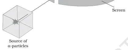
Introduction: In the Rutherford (alpha‑particle) scattering experiment, a narrow beam of high‑energy alpha particles (He2+) was directed at a very thin metal foil (e.g. gold). Detectors (scintillation screen or photographic plate) around the foil recorded the angular distribution of scattered alpha particles. The experiment (1909–1911) led to the nuclear model of the atom.

Experimental setup:

• Alpha source (Polonium/Radium) producing mono‑energetic alpha particles.
• Slits/collimators to form a narrow beam.
• Thin metal foil (typically gold) as the target.
• Rotatable detector (ZnS scintillator / photographic plate) to count scattered alphas at different angles θ.

Key observations:

• Most alpha particles passed through the foil with little or no deflection — atom is mostly empty space.
• A small fraction were deflected by large angles; a very few were backscattered (θ > 90°) — implies a very small, massive center of positive charge.
• The number of particles scattered into angle θ followed a distribution that fell steeply with θ; quantitative agreement with Coulomb scattering (Rutherford formula) was found.

Conclusions (Rutherford model):

• Atomic positive charge and most of the atomic mass are concentrated in a very small region called the nucleus (size ≈ 10^−14 to 10^−15 m).
• Electrons move around the nucleus; most of the atom’s volume is empty space.
• The nucleus has charge +ZNe (ZN = atomic number) and exerts Coulomb repulsion on alpha particles (Zα = 2).

Physical picture & classical analysis: The scattering is due to repulsive Coulomb force between the positive alpha (projectile charge +Z1e) and the target nucleus (+Z2e). Classical trajectories (hyperbolas) give relations between impact parameter b and scattering angle θ, and the differential cross‑section dσ/dΩ, which depends strongly on θ (∝ 1/sin^4(θ/2)).

Limitations: The classical Rutherford formula assumes purely Coulomb interaction, pointlike nucleus, non‑relativistic projectiles and a stationary heavy nucleus (no nuclear forces). At very small distances (high energies) nuclear forces and quantum/relativistic effects become important.

Significance: Rutherford’s experiment overturned the Thomson "plum pudding" model and established the nuclear atom; it also provided a method (Rutherford backscattering) for probing nuclear charge and thin‑film composition.

Fig 12.3 — Educational Diagram: Limitations of Rutherford model

Summary: Rutherford's nuclear model (heavy positive nucleus with electrons orbiting like planets) explained α-particle scattering but failed to account for several observed atomic properties. Major limitations arise because it treats orbiting electrons classically.

1. Instability of the atom (radiation loss):

   According to classical electrodynamics, an accelerated charge radiates electromagnetic energy. An electron in a circular orbit around the nucleus is constantly accelerating (centripetal acceleration) and so should continuously lose energy, spiral inward and collapse into the nucleus in a very short time. Rutherford's model gives no mechanism to prevent this.

   Brief estimate using the Larmor formula (non‑relativistic):

   P = (e^2 a^2) / (6πε₀ c^3), where a = v^2 / r and v^2 = e^2 / (4πε₀ m r) from Coulomb force.

   For r ≈ 5.3×10⁻¹¹ m (Bohr radius) this gives P ≈ 10⁻⁸ W and the orbital energy ≈ 2.18×10⁻¹⁸ J. Time to radiate that energy t ~ E/P ≈ 10⁻¹¹ s. So classically the atom would be unstable.

2. Cannot explain discrete (line) spectra:

   Rutherford's model predicts a continuously varying electron energy as it spirals toward the nucleus, so the emitted radiation should form a continuous spectrum. Experimentally atoms (e.g., hydrogen) show sharp, discrete spectral lines (Balmer, Lyman series etc.). Rutherford's model cannot predict these quantized energies or the wavelengths of spectral lines.

3. No quantization or explanation of chemical/periodic behavior:

   The model does not specify allowed electron energies, shells or configurations, so it cannot explain the periodicity of elements, valency, or chemical properties that depend on discrete electron states.

4. No account of atomic fine structure, spin and spectroscopic details:

   Phenomena like fine and hyperfine spectral splitting, electron spin, Zeeman effect and Lamb shift require quantum mechanics and additional structure not present in Rutherford’s picture.

5. Electron distribution and size issues:

   The model treats electrons as point particles moving in well-defined classical orbits; it gives no probabilistic electron-cloud picture or explanation of atomic radii that quantum theory provides.

Historical consequence: These failures motivated the Bohr model and, later, full quantum mechanics (Schrödinger, Heisenberg) which introduce quantized energy levels, stationary states that do not radiate, and probability distributions for electrons—successfully explaining spectral lines and atomic stability.

Fig 12.4 — Educational Diagram: Atomic spectra

Atomic spectra are the characteristic patterns of electromagnetic radiation (light) emitted or absorbed by atoms when their electrons change energy levels. They arise because electrons in atoms occupy quantized energy levels; a transition from a higher level to a lower level emits a photon, and a transition from a lower to a higher level requires absorption of a photon of that exact energy.

Types of spectra

• Continuous spectrum: produced by dense hot objects (e.g., incandescent solids) — all wavelengths are present.
• Emission (line) spectrum: produced by hot, low-density gases — discrete bright lines at specific wavelengths (each line = a transition).
• Absorption spectrum: when a cooler gas lies in front of a continuous source; dark lines appear where photons were absorbed to excite atoms.

Origin (qualitative): For hydrogen-like atoms the allowed energies are discrete. A transition from level n_i to n_f (n_i > n_f) emits a photon of energy equal to the difference of the two levels: E_photon = E_{n_i} - E_{n_f}. The corresponding wavelength λ satisfies E_photon = hν = hc/λ.

Bohr model (useful for hydrogen and hydrogen-like ions): Energy levels (in electronvolts) are given by E_n = -13.6 eV × (Z^2 / n^2), where Z is nuclear charge and n = 1, 2, 3,... Transitions between levels give the line (Rydberg) formula for wavelengths:

1/λ = R × Z^2 × (1/n_f^2 - 1/n_i^2)

where R = 1.097373 × 10^7 m^-1 (Rydberg constant), n_i > n_f.

Series in hydrogen: groups of lines corresponding to fixed n_f:

• Lyman series: n_f = 1 (ultraviolet)
• Balmer series: n_f = 2 (visible — e.g., Hα at 656.3 nm)
• Paschen: n_f = 3 (infrared)

Selection rules and fine details: The dominant electric-dipole selection rule is Δl = ±1 (change in orbital quantum number). Real spectra show fine structure (spin–orbit splitting), hyperfine structure (nuclear interactions), Zeeman/Stark splitting in fields, and broadening mechanisms (natural, Doppler, collisional/pressure).

Kirchhoff’s spectroscopic laws (practical rules):

• Hot dense body → continuous spectrum.
• Hot low-density gas → emission line spectrum.
• Cool gas in front of a continuous source → absorption line spectrum.

Importance & applications: Atomic spectra provide fingerprints of elements — used in astronomical spectroscopy (identifying stellar composition and redshift), laboratory spectroscopy, flame tests, neon signs, sodium-vapor lamps, and in precise measurements (atomic clocks).

Fig 12.5 — Educational Diagram: Bohr model of the hydrogen atom

Overview
Bohr's model (1913) explains the discrete spectral lines of hydrogen by postulating that the electron moves in certain allowed circular orbits without radiating energy and that radiation is emitted or absorbed only when the electron jumps between these orbits.

Bohr's postulates

• Electrons move in circular orbits under Coulomb attraction but do not radiate while in a permitted (stationary) orbit.
• Only certain orbits are allowed: the angular momentum of the electron is quantized: L = mvr = nħ, where n = 1, 2, 3, ... and ħ = h/2π.
• Radiation is emitted or absorbed when an electron jumps between two allowed orbits. The frequency ν of the photon is given by ΔE = E_i − E_f = hν.

Key results (for hydrogen / hydrogen-like ions)

• Allowed radii: r_n = a_0 n^2, where a_0 (Bohr radius) = 4πε_0 ħ^2/(m_e e^2) ≈ 0.529 × 10⁻¹⁰ m.
• Allowed energies: E_n = −13.6 eV / n^2 (for hydrogen). Energies are negative (bound states) and approach 0 from below as n → ∞.
• Photon frequency on transition n_i → n_f (n_i > n_f): hν = E_{n_i} − E_{n_f} ⇒ 1/λ = R_H (1/n_f^2 − 1/n_i^2), where R_H ≈ 1.097 × 10⁷ m⁻¹ (Rydberg constant for H).

Brief derivation (outline)

1. Balance forces: Coulomb force = centripetal force ⇒ (1/4πε_0)(e^2/r^2) = m_e v^2/r.
2. Use quantization m_e v r = nħ to eliminate v; solve for r to get r_n = (4πε_0 ħ^2)/(m_e e^2) n^2 = a_0 n^2.
3. Total energy = K + U = (1/2)m_ev^2 − (1/4πε_0)(e^2/r) = −(1/8πε_0)(m_e e^4/ħ^2)(1/n^2) = −13.6 eV/n^2.

Spectral series
Different series arise from transitions ending at fixed n_f: Lyman (n_f = 1, ultraviolet), Balmer (n_f = 2, visible), Paschen (n_f = 3, infrared), etc.

Limitations
Bohr model correctly predicts hydrogen-like spectra but fails for multi-electron atoms, cannot explain fine structure, Zeeman splitting, or intensities and selection rules fully. It was superseded by quantum mechanics (Schrödinger wave mechanics and quantum electrodynamics).

Fig 12.6 — Educational Diagram: Applications and examples

Overview
Bohr's model and the quantum description of atoms explain discrete energy levels in atoms. These quantized levels lead to emission and absorption of photons with specific wavelengths, forming the basis of atomic spectroscopy. Applications range from identifying elements to precision timekeeping and astrophysical measurements.

Key applications

• Spectroscopy and chemical analysis: Emission/absorption spectra uniquely identify elements (flame tests, emission tubes, laboratory spectrometers).
• Astronomy: Stellar spectra reveal chemical composition, temperature and redshift (Doppler shift of spectral lines).
• X-ray spectroscopy & Moseley’s law: Characteristic X-rays identify elements and confirm atomic number ordering.
• Lasers and LEDs: Atomic and ionic transitions are exploited to generate coherent or monochromatic light.
• Atomic clocks: Hyperfine transitions in atoms (e.g., Cs-133) provide extremely stable frequency standards.
• Determination of fundamental constants: Spectral lines allow precise measurement of the Rydberg constant; reduced-mass corrections refine values.
• Experimental confirmation of quantization: Franck–Hertz experiment and discrete line spectra confirm energy quantization.

Limitations & refinements
Bohr model works well for hydrogen-like atoms (single electron). For multi-electron atoms and fine details (fine structure, hyperfine splitting, Lamb shift) full quantum mechanics (Schrödinger/Dirac equations, electron-electron interaction) is required.

Fig 12.7 — Educational Diagram: Successes and shortcomings of Bohr model

Introduction: The Bohr model (1913) introduced quantized electron orbits for the hydrogen atom. It postulated that electrons move in certain allowed circular orbits without radiating energy (stationary states) and that radiation is emitted or absorbed when an electron jumps between these orbits. The model uses angular momentum quantization: mvr = nħ (n = 1,2,...).

Major successes:

• Explanation of hydrogen spectral lines: Bohr derived the Rydberg formula for wavelengths of spectral lines of hydrogen and hydrogen-like ions, giving excellent agreement with experimental spectra (Balmer, Lyman, Paschen series etc.).
• Quantitative energy levels: The expression for energy levels, E_n = -13.6 eV (Z^2/n^2), correctly predicts ionization energy and line positions for hydrogen and hydrogen-like one-electron ions (He+, Li2+).
• Bohr radius and atomic size: The model gives a definite ground-state radius a0 ≈ 0.529 × 10^-10 m, a useful estimate of atomic size.
• Bohr frequency condition and correspondence principle: The frequency of emitted/absorbed radiation obeys hν = E_i − E_f. For large n the model recovers classical results (correspondence principle).
• Simple physical picture: Provides an intuitive, semi-classical picture of quantization that helped development of quantum theory.

Important derived relations (used in successes): radius r_n ∝ n^2, energy E_n ∝ −1/n^2, and the Rydberg formula for λ. These relations allow direct calculation of spectral lines and atomic radii for hydrogenic systems.

Shortcomings and limitations:

• Fails for multi-electron atoms: Bohr model cannot account for electron–electron interactions or complex spectra of atoms with more than one electron.
• No explanation of spectral line intensities: The model predicts only line positions, not relative intensities or selection rules correctly.
• Cannot explain fine structure, spin, and relativistic effects: It does not include electron spin or relativistic corrections (fine structure) and cannot explain the Lamb shift or hyperfine structure.
• Zeeman and Stark effects: The model cannot fully describe splitting patterns in magnetic (Zeeman) and electric (Stark) fields except by ad hoc modifications.
• Assumes circular orbits and classical trajectories: The model uses fixed circular orbits whereas electrons have wave nature; it conflicts with uncertainty principle and fails for non-circular motion.
• Inconsistent foundations: Mixing of classical mechanics (orbits) with quantization rules is conceptually unsatisfactory and replaced by wave mechanics (Schrödinger) and quantum mechanics.

Conclusion: Bohr model was a crucial step: it successfully explained hydrogen-like spectra quantitatively and introduced quantization ideas, but it is incomplete. Modern quantum mechanics (wavefunctions, operators, and Pauli spin) overcomes all its shortcomings and gives a consistent, general description.

Fig 12.8 — Educational Diagram: Summary and key formulae

Brief summary: This topic reviews atomic models leading to the Bohr model for hydrogen-like atoms and the key formulae that describe their radii, energies and spectra. Rutherford scattering showed a compact positive nucleus but could not explain atomic stability or discrete spectral lines. Bohr introduced quantization of angular momentum and energy to explain hydrogen spectra.

Bohr model — main ideas:

• Electrons move in circular orbits under Coulomb attraction. Only certain orbits are allowed; angular momentum is quantized: m v r = n ħ, where n = 1, 2, 3, ...
• Energy of an electron in an allowed orbit is discrete (E_n). Radiation (photon) is emitted or absorbed when an electron jumps between orbits: hν = E_i − E_f.
• The model works very well for hydrogen and hydrogen-like (single-electron) ions (He+, Li2+, ...), and gives the Rydberg formula for spectral lines.

Physical consequences: Orbit radii increase as n^2; energy levels scale as −1/n^2 (they get closer for large n). Transition energies give the observed spectral series (Lyman, Balmer, Paschen, ...). Reduced-mass correction improves precision for real atoms. Bohr model has limitations (fails for multi-electron atoms, fine structure, Zeeman effect, etc.) but remains useful for basic spectra and estimates.

Important constants and typical numerical values:

• Bohr radius: a₀ = 4πε₀ħ²/(m_e e²) = 5.29 × 10⁻¹¹ m
• Ground-state energy of H: E₁ = −13.6 eV
• Rydberg constant: R_∞ = 1.097373 × 10⁷ m⁻¹ (use reduced-mass corrected R ≈ R_∞ μ/m_e)
• Fine-structure constant: α ≈ 1/137
• Bohr magneton: μ_B = eħ/(2m_e) = 9.274 × 10⁻²⁴ J/T

Where it appears in real life: Atomic emission and absorption spectra are used in chemical analysis (spectroscopy), astrophysics (stellar composition and redshift), gas-discharge lamps and neon signs (characteristic emission lines), and in teaching basic quantum ideas. Hydrogen spectral lines (Balmer series) are visible in astronomical spectra and laboratory discharge tubes.