Overview
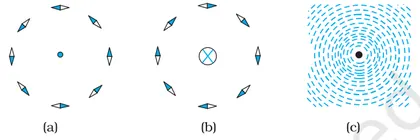
This chapter explores magnetism produced by moving electric charges and steady currents, and the forces and motions that result when charges or current-carrying conductors are placed in magnetic fields. It builds on electrostatics and introduces magnetic field as a vector field, the Biot–Savart law and Ampère's circuital law for calculating magnetic fields, and the Lorentz force law for force on moving charges and on current elements. The chapter is important because it explains the physical principles behind electric motors, galvanometers, cyclotrons, mass spectrometers and other electromagnetic devices, and develops vector and integral calculus skills used throughout physics. Students will learn to apply right-hand rules, perform simple Biot–Savart and Ampère-law calculations (long straight wire, circular loop, solenoid), analyse motion of charged particles in uniform magnetic fields (circular and helical trajectories), compute force and torque on current loops (magnetic dipole moment and potential energy), and use these ideas in practical contexts such as velocity selectors, cyclotrons and basic magnetic measurement devices.
Learning Objectives
- Define magnetic force on a moving charge and state the Lorentz force law for a charge moving in combined electric and magnetic fields.
- Explain the direction of magnetic force using the right-hand rule and predict the deflection of positive and negative charges in a uniform magnetic field.
- Derive the expression for the radius and frequency of circular motion of a charged particle moving perpendicular to a uniform magnetic field and apply it to solve numerical problems.
- Determine the trajectory (circular, helical or straight) of a charged particle for given initial velocity components in a uniform magnetic field.
- State and derive the magnetic force on a current-carrying conductor (F = I L × B) and apply it to calculate forces in typical exam problems.
- Calculate the force between two long parallel current-carrying conductors and use the result to define the ampere and explain like/unlike current interactions.
- Explain and apply the Biot–Savart law to obtain the magnetic field on the axis of a current loop and near a finite straight wire (solve related numericals).
- State Ampère's circuital law and apply it to determine magnetic fields of highly symmetric configurations (long straight wire, solenoid, toroid) in exam-type questions.
Topics in this chapter
12 topics · tap a topic title to jump straight to it.
Magnetic force on a moving charge
Definition: A charge q moving with velocity v in a magnetic field B experiences a magnetic force given by the Lorentz law: the magnetic part is F = q (v × B). This is a vector (cross) product so the force is perpendicular to both v and B.
Magnitude: |F| = q v B sinθ, where θ is the angle between v and B. For a positive charge the direction is given by the right‑hand rule (point fingers along v, curl toward B; thumb gives F). For a negative charge the force is opposite.
Special orientations:
- v parallel (or antiparallel) to B (θ = 0 or π): sinθ = 0 → F = 0 → the magnetic field does not affect the motion.
- v perpendicular to B (θ = 90°): maximum force → particle moves in a circle.
- v at an oblique angle: motion is a helix (circular motion in the plane perpendicular to B combined with uniform motion parallel to B).
Circular motion (v ⟂ B): The magnetic force provides centripetal force: q v B = m v^2 / r, so the radius of the circle is r = m v / (q B). The angular (cyclotron) frequency is ω = q B / m and the period is T = 2π m / (q B).
Helical motion: Resolve velocity into v⊥ and v∥ (perp and parallel to B). v⊥ causes circular motion of radius r = m v⊥/(qB); v∥ is uniform motion along B. Pitch (distance advanced per revolution) = v∥ T.
Work and energy: Magnetic force is always perpendicular to instantaneous velocity, so it does no work: W = ∫F·ds = 0. Consequently the speed (and kinetic energy) of the charge remains constant; only the direction changes.
Relation to current: For a current element i dL, dF = i (dL × B). For a straight conductor of length L carrying current i in a uniform B: F = i L B sinθ (direction given by right-hand rule i × B).
Combined electric and magnetic fields: Full Lorentz force is F = q(E + v × B). In crossed E and B fields a velocity selector uses E = v B to allow only particles with speed v = E/B to pass straight.
Key conceptual points:
- Magnetic force changes only direction of velocity, not its magnitude.
- Direction depends on sign of charge; negative charges are deflected opposite to the right‑hand rule.
- Magnetic fields do not pull charges toward or away unless there is a velocity component causing a transverse force.
- Cyclotron / synchrotron: charged particles follow circular or spiral paths in magnetic fields; cyclotron frequency ω = qB/m sets the orbital frequency.
- Mass spectrometer: magnetic deflection separates ions by mass/charge ratio because r = m v /(q B).
- Cathode ray tube (CRT): electrons are deflected by magnetic fields to steer the beam.
- Velocity selector: crossed electric and magnetic fields allow only particles with v = E/B to pass undeviated.
- Electric motor / loudspeaker: force on current-carrying conductors (F = i L × B) produces torque and motion.
- Lorentz magnetic force (vector): F = q (v × B)
- Magnitude: |F| = q v B sinθ
- Circular motion radius (v ⟂ B): r = m v /(q B)
- Cyclotron angular frequency: ω = q B / m
- Cyclotron frequency (Hz): f = q B /(2π m)
- Period: T = 2π m /(q B)
Motion of charged particles in uniform magnetic and combined fields
Basic law (Lorentz force): A charge q moving with velocity v in electric field E and magnetic field B experiences force F = q(E + v × B). In the absence of E, the magnetic part is F_B = q(v × B). The magnetic force is always perpendicular to v and B, does no work and changes only the direction of v.
Uniform magnetic field only (E = 0):
- If v ⟂ B (velocity fully perpendicular to B): the magnetic force has magnitude F = qvB and is centripetal. The particle undergoes uniform circular motion with radius r = mv/(|q|B). The angular (cyclotron) frequency is ω = |q|B/m and period T = 2πm/(|q|B). Speed |v| stays constant.
- If v ∥ B (velocity parallel to B): v × B = 0, so there is no magnetic force; the particle moves in a straight line at constant speed along B.
- If v makes angle θ with B: decompose v = v_∥ + v_⊥. The parallel component v_∥ remains unchanged; the perpendicular component v_⊥ produces circular motion about the field lines. The overall path is a helix with radius r = m v_⊥/(|q|B). The pitch (advance per turn) p = v_∥ T = 2π m v_∥/(|q|B).
- Direction: use right-hand rule for positive charges (thumb along v, fingers toward B, force is palm direction of v × B). For negative charges, force is opposite.
Uniform combined (E and B) fields:
- General force: F = q(E + v × B). The motion is determined by both fields; magnetic component is velocity dependent and does not change kinetic energy, while the electric component can accelerate the particle.
- Case E ∥ B: electric force qE accelerates the particle along the field; magnetic force acts on perpendicular velocity components only, so motion can be a combination of longitudinal acceleration and perpendicular circular/helix motion.
- Case E ⟂ B (crossed fields): two important subcases:
- Velocity selector (E and B perpendicular and set so E = vB): particles with v = E/B experience q(E + v × B) = 0 and go undeflected — used to select particles of a specific speed.
- E × B drift: in a uniform crossed field, every charged particle (regardless of sign and mass) drifts with velocity v_d = E × B / B^2. This drift is perpendicular to both E and B and is independent of particle charge and speed.
Important physical points: magnetic field alone cannot change a particle's speed, only its direction; radius of curvature increases with momentum and decreases with magnetic field strength; crossed E and B allow control of trajectories (selection, confinement, and drift). These principles underlie mass spectrometers, cyclotrons, velocity selectors, cathode-ray tubes and magnetic confinement devices.
- Cyclotron: uses perpendicular magnetic field to bend charged particles into circular orbits; increasing energy makes radius grow as r = mv/(qB).
- Mass spectrometer: ions in a magnetic field follow circular arcs; the radius depends on m/q and momentum, allowing separation by mass-to-charge ratio.
- Velocity selector (Thomson’s crossed-field apparatus): only particles with v = E/B pass straight through undeflected.
- Cathode-ray tube / old TV and oscilloscopes: electrons deflected by magnetic (and electric) fields to form images.
- Aurora and charged-particle motion in Earth’s magnetic field: charged particles spiral along geomagnetic field lines (helical motion) and precipitate in upper atmosphere producing auroras.
- Tokamak / magnetic confinement in fusion: charged plasma particles spiral along and drift across field lines; magnetic fields confine hot plasma.
- Lorentz force: F = q(E + v × B)
- Magnetic force magnitude: |F_B| = |q| v B sinθ
- Centripetal condition (v ⟂ B): |q| v B = m v^2 / r → r = m v / (|q| B)
- Cyclotron angular frequency: ω = |q| B / m
- Cyclotron period: T = 2π m / (|q| B)
- Helix pitch: p = v_∥ T = 2π m v_∥ / (|q| B)
Force on a current-carrying conductor in a magnetic field
Definition: A current-carrying conductor placed in a magnetic field experiences a force due to the magnetic field acting on the moving charge carriers. This phenomenon is the basis of electric motors and many electromagnetic devices.
Microscopic cause (Lorentz force): A charge q moving with velocity v in a magnetic field B experiences the Lorentz force F = q (v × B). In a conductor, the charge carriers (electrons) have drift velocity v_d, so each carrier feels q (v_d × B).
Macroscopic force on a conductor (derivation outline): For a straight conductor of length L and cross-sectional area A carrying current I, the current density relation I = n q A v_d (where n is number density of carriers) can be used. The total magnetic force on all charges in the segment of length L becomes F = I (L × B). In vector form for a straight segment:
F = I L × B
Magnitude: F = I L B sin θ, where θ is the angle between the direction of the current (vector L) and the magnetic field B. Direction: given by Fleming's left-hand rule (for conventional current) or by the right-hand rule for the vector cross product.
General element form: For a conductor of arbitrary shape, an infinitesimal element dl carrying current I experiences dF = I (dl × B). The total force is F = ∫ I (dl × B).
Special cases and features:
- If current is parallel to B (θ = 0°), F = 0.
- If current is perpendicular to B (θ = 90°), F = I L B (maximum).
- Magnetic forces are always perpendicular to the instantaneous velocity of charges, so magnetic field alone does no work on a free charge. In circuits, however, mechanical work can be extracted (motor action) because of interactions between fields and the lattice/contacts.
Force between two parallel currents: Two long, straight, parallel conductors separated by distance r carrying currents I1 and I2 exert magnetic forces on each other. The magnitude of force per unit length on each is
F/L = (μ0 I1 I2) / (2π r)
Like currents attract; opposite currents repel. This relation is used to define the ampere in terms of force between conductors.
Torque on a current loop (motor principle): A rectangular coil or loop of area A carrying current I in a uniform magnetic field B experiences a torque τ = N I A B sin φ, where N is number of turns and φ is the angle between the loop normal and B. This torque is the operating principle of electric motors.
Units: Force (F) in newtons (N); magnetic field B in tesla (T); I in amperes (A); length L in meters (m). 1 T = 1 N·s / (C·m) equivalently N/(A·m).
Practical note: The magnitude relations and direction rules are essential for designing motors, loudspeakers, galvanometers and for analyzing forces in power devices. In experiments, Fleming's left-hand rule gives a quick way to find the direction of force on a conductor.
- DC electric motor: current in coils within a magnetic field experiences torque — converts electrical energy to mechanical energy.
- Loudspeaker: current in a coil in the magnetic gap produces a force that moves the diaphragm to create sound.
- Moving-coil galvanometer: small current in a coil produces a torque and deflection proportional to current.
- Railgun: large currents in parallel rails produce strong magnetic forces that accelerate a projectile.
- Maglev (magnetic levitation) and braking: forces between currents and fields are used for levitation or contactless braking (eddy-current braking).
- Deflection of electron beam in CRT: moving electrons (current) in magnetic field are deflected by Lorentz force.
- Lorentz force on a charge: F = q (v × B)
- Force on a straight conductor (vector): F = I (L × B)
- Magnitude for straight conductor: F = I L B sin θ
- Infinitesimal element: dF = I (dl × B) and F = ∫ I (dl × B)
- Force per unit length between parallel currents: F/L = μ0 I1 I2 / (2π r)
- Torque on N-turn coil of area A: τ = N I A B sin φ
Biot–Savart law and magnetic field due to current elements
What it states
The Biot–Savart law gives the magnetic field produced at a point in space by a small element of steady current. For a current element of magnitude I and length vector dℓ, the differential magnetic field dB at a point located by the vector r (from the element to the point) is
dB = (μ0 / 4π) (I dℓ × r̂) / r2
or equivalently using vector r (not unit vector),
dB = (μ0 / 4π) (I dℓ × r) / r3
Here μ0 = 4π × 10−7 T·m/A is the permeability of free space, r = |r| is the distance from the current element to the field point, and r̂ is the unit vector from the element to the point. The magnitude of the contribution is
dB = (μ0 / 4π) (I dℓ sinθ) / r2
where θ is the angle between dℓ and r̂. The direction of dB is given by the right-hand rule for the cross product (point thumb along current, fingers toward the field point, and the curled direction gives the magnetic field direction).
Superposition and magnetostatics
The total field B is the vector integral over the entire current distribution: B = ∫ dB. Biot–Savart applies for steady (time-independent) currents and is the magnetostatics analogue of Coulomb's law for electric fields.
Common worked results (special cases)
- Infinite straight wire: Using Biot–Savart and symmetry, for a long straight wire carrying current I, the magnetic field at perpendicular distance r is
B = μ0 I / (2π r)Direction: concentric circles around the wire (right-hand rule).
- Finite straight wire: If the wire subtends angles α and β at the field point (measured from the point to the two ends),
B = (μ0 I / 4π r) (sin α + sin β)(r is perpendicular distance to the wire).
- Circular loop (on axis): For a circular loop radius R carrying current I, the magnetic field at a point on the axis a distance x from the center is
B(x) = (μ0 I R2) / (2 (R2 + x2)3/2)At the centre (x = 0): B = μ0 I / (2R).
- Coil with N turns / long solenoid: Multiply the single-loop result by N for N closely spaced turns. For an ideal long solenoid with turn density n (turns per metre), B inside ≈ μ0 n I (uniform along axis).
Direction rules and visualization
The right-hand rule: curl fingers in the direction of current; thumb gives the direction of dℓ × r̂ (or point thumb along current and the curling of fingers shows the circular field lines). Field lines around straight conductors are closed circles.
Assumptions & limitations
Biot–Savart applies to steady currents (no changing electric fields). For time-varying fields Maxwell’s correction (displacement current) must be included via Ampère–Maxwell law.
Why important
Biot–Savart is the fundamental relation used to calculate magnetic fields from any current shape, and yields many standard textbook results (fields of wires, loops, coils) that describe real devices like motors, inductors and magnetic sensing equipment.
- Magnetic field around a long straight power-carrying transmission line — use B = μ0 I / (2π r) to estimate field strength at ground level.
- Field at the center of a circular coil used in MRI gradient coils — B_center = μ0 I / (2R) (for one loop) and multiply by number of turns.
- Inside a solenoid (electromagnet) used in door locks and loudspeakers — B ≈ μ0 n I gives approximately uniform field along the axis.
- Direction of needle deflection in a compass near a current-carrying wire — predicted by the right-hand rule and Biot–Savart field lines.
- Differential (vector) form: dB = (μ0 / 4π) (I dℓ × r̂) / r^2
- Differential (vector, using r): dB = (μ0 / 4π) (I dℓ × r) / r^3
- Magnitude of differential: dB = (μ0 / 4π) (I dℓ sinθ) / r^2
- Infinite straight wire: B(r) = μ0 I / (2π r)
- Finite straight wire: B = (μ0 I / 4π r) (sin α + sin β)
- Circular loop on axis: B(x) = (μ0 I R^2) / (2 (R^2 + x^2)^(3/2)); at center x=0: B = μ0 I / (2R)
Ampère's circuital law and its applications
Statement (integral form): The line integral of the magnetic field B around a closed path (Amperian loop) is equal to μ0 times the net steady current I_enc that passes through any surface bounded by that path:
∫ B · dl = μ0 Ienc
Physical meaning: Currents produce circulation of the magnetic field. Ampère's law relates that circulation (integral of B along a closed curve) to the total current pierced by the curve.
Differential form: Using Stokes' theorem, Ampère's law becomes the curl form:
∇ × B = μ0 J
(J is current density). This is useful in Maxwell's equations and local field analysis.
Maxwell correction (advanced note): For time-varying electric fields, Maxwell added the displacement current term, giving
∫ B · dl = μ0 Ienc + μ0ε0 dΦE/dt
This general form is required when currents vary with time (e.g., charging capacitors). In steady currents the displacement term is zero and the simpler form applies.
How to apply Ampère's law (procedure):
- Identify symmetry (cylindrical, planar, or toroidal) so B is constant on chosen segments and either parallel or perpendicular to dl.
- Choose an Amperian loop consistent with the symmetry (circle for long straight wire, rectangle for solenoid, concentric circle for toroid).
- Compute the integral ∫ B · dl = B × (path length where B is parallel to dl).
- Determine I_enc (total current passing through the surface bounded by the loop).
- Solve for B.
Common class-12 applications:
- Infinite straight long wire (cylindrical symmetry): Using a circular Amperian loop of radius r centered on the wire one gets B(r) = μ0 I / (2π r). Field lines are concentric circles around the wire; direction by right-hand rule.
- Long ideal solenoid (axial symmetry): For a tightly wound solenoid of n turns per unit length carrying current I, inside B = μ0 n I (uniform and parallel to axis). Outside (ideal infinite solenoid) B ≈ 0.
- Toroid (circular symmetry): For a toroid with N turns carrying I, at radial distance r (within the core) B(r) = μ0 N I / (2π r). Outside the torus B = 0 (no net current enclosed by an external loop).
- Infinite current sheet: For a large flat sheet with surface current density K, the magnetic field on each side has magnitude B = (μ0 K)/2 and changes sign across the sheet.
- Force between two parallel currents: Use Ampère's law to get B from one wire and then Lorentz force on the other to derive F/L = μ0 I1 I2 / (2π d) (attraction for same direction currents).
Limitations and tips: Ampère's law is most useful when there is high symmetry allowing B to be taken constant over parts of the chosen loop. For arbitrary current distributions you may need Biot–Savart law or use the differential form with boundary conditions.
- MRI magnets: large superconducting solenoids produce a very uniform axial magnetic field inside the bore, designed using B = μ0 n I (solenoid approximation).
- Toroidal inductors and transformers in electronics: toroid geometry confines magnetic field inside the core (B ∝ 1/r), reducing external interference.
- Power transmission lines and magnetic fields: long straight conductors produce circular B-fields (B = μ0 I / 2πr); the interaction of parallel lines gives forces used to define the ampere.
- Electromagnets and loudspeakers: coils (solenoids) with iron cores create concentrated magnetic fields that produce forces on magnets or current-carrying conductors.
- Current sheets in plasma physics and Hall-effect devices: idealized planar current distributions are analyzed with Ampère's law to find field jumps across the sheet.
- Integral form: ∮ B · dl = μ0 I_enc
- Differential form: ∇ × B = μ0 J
- Maxwell-corrected form (time-varying fields): ∮ B · dl = μ0 I_enc + μ0 ε0 dΦ_E/dt
- B around an infinitely long straight wire: B(r) = μ0 I / (2π r)
- B inside an ideal long solenoid: B = μ0 n I (n = N/L, number of turns per unit length)
- B inside a toroid (at radius r): B(r) = μ0 N I / (2π r)
Magnetic field of common current configurations
Overview. Moving electric charges (steady currents) produce magnetic fields. Two fundamental tools to calculate these fields are the Biot–Savart law (for direct calculation from current elements) and Ampère's circuital law (useful when there is symmetry). The direction of the magnetic field B produced by a current I is given by the right‑hand rule: thumb along current, curled fingers show the field lines.
Fundamental relations.
- Biot–Savart law: dB = (μ0 / 4π) * (I dl × r̂) / r^2. Integrate over the conductor to get B at the observation point. (μ0 = 4π × 10−7 T·m/A in vacuum.)
- Ampère's law (steady currents): ∮ B · dl = μ0 I_enc. Useful when B has high symmetry (e.g., infinite straight wire, infinite solenoid, current sheet).
Common current configurations (direction and magnitude):
- Infinite straight long wire: Field circles the wire. Magnitude at distance r from the wire:
B = μ0 I / (2π r)
Use right‑hand rule to get direction (azimuthal). - Finite straight segment: If the wire extends from angles θ1 to θ2 as seen from the field point, the Biot–Savart result is
B = (μ0 I / 4π r) (sin θ1 + sin θ2)
Special cases: semi‑infinite wire gives B = μ0 I / (4π r), infinite wire reduces to μ0 I / (2π r). - Circular loop (single turn):
- At the center (radius R): B_center = μ0 I / (2 R) (direction along axis, given by right‑hand rule).
- On axis at distance x from center: B(x) = (μ0 I R^2) / [2 (R^2 + x^2)^(3/2)]. For N turns, multiply by N.
- Solenoid (long, closely wound):
Inside (approx. uniform): B = μ0 n I, where n = N/L is the number of turns per unit length. Direction along solenoid axis given by right‑hand rule. Outside (ideal infinite solenoid): B ≈ 0.
Edge effects make B vary near the ends (fringing fields). - Toroid (circular ring of N turns):
Inside the ring at radius r (between inner and outer core boundaries): B = μ0 N I / (2π r). Outside an ideal toroid B ≈ 0 (field confined inside).
- Infinite current sheet (surface current density K):
Magnetic field on each side is constant in magnitude: B = μ0 K / 2 (direction given by right‑hand rule around current direction).
Direction and superposition. Magnetic fields obey superposition—fields from multiple current elements add vectorially. Use right‑hand/fleming rules to determine directions and symmetry arguments or Ampère’s law to find magnitudes where applicable.
Practical notes. Real coils and solenoids are finite: fields are not perfectly uniform and have fringing near ends. Materials with high magnetic permeability (iron cores) concentrate field lines and increase B for the same current.
- Compass deflection near a current‑carrying wire (demonstrates circular B around a straight wire).
- Electromagnet (solenoid with ferromagnetic core) used in cranes and relays — solenoid produces strong nearly uniform axial B inside coil.
- Loudspeaker coil (voice coil) — current through coil in magnetic field produces force; coil geometry is often circular/solenoidal.
- Toroidal transformers and inductors — toroidal windings confine magnetic field, reducing external flux and interference.
- MRI gradient coils and imaging — use carefully designed coil geometries to produce known magnetic field profiles (uniform inside, controlled gradients).
- Biot–Savart law: dB = (μ0 / 4π) * (I dl × r̂) / r^2
- Ampère's law: ∮ B · dl = μ0 I_enc
- Infinite straight wire: B = μ0 I / (2π r)
- Finite straight segment (angles θ1, θ2): B = (μ0 I / 4π r) (sin θ1 + sin θ2)
- Circular loop on axis: B(x) = (μ0 I R^2) / [2 (R^2 + x^2)^(3/2)] ; center (x=0): B = μ0 I / (2 R)
- Solenoid (long): B = μ0 n I = μ0 (N/L) I (inside, approximately uniform)
Force between two parallel currents
What it is
When two long, straight, parallel conductors carry steady currents, each conductor produces a magnetic field that acts on the other. The interaction produces a magnetic force per unit length between them: currents in the same direction attract, currents in opposite directions repel.
Derivation (concise)
Consider two long straight wires separated by distance d carrying currents I1 and I2. The magnetic field at distance r from a long straight wire (by Ampère/Biot–Savart) is B = μ0 I /(2π r), directed azimuthally around the wire (right‑hand rule). At the position of the second wire (r = d) the field from wire 1 is B1 = μ0 I1 /(2π d). The magnetic force on a length L of wire 2 is F = I2 L × B1 (here the angle is 90°), so
F = I2 L B1 = μ0 I1 I2 L /(2π d)
Therefore the magnitude of force per unit length is
F/L = μ0 I1 I2 /(2π d)
Direction
Use the right‑hand rule for the field around wire 1 and the force law F = I (L × B): if currents are parallel (same direction) the force is attractive (wires pulled together); if currents are antiparallel the force is repulsive.
Conditions & notes
This formula assumes long (effectively infinite) straight conductors, steady currents, and separation much larger than wire radii. In a material medium replace μ0 by μ = μ0 μr. Historically, the ampere was defined using the force between two parallel currents: two ideal parallel conductors 1 m apart in vacuum, each carrying 1 A, exert a force of 2×10^−7 N per metre on each other (which gives μ0 = 4π×10^−7 T·m/A).
- Overhead power transmission lines: parallel conductors carrying large currents experience measurable attraction or repulsion; wind and current differences can cause lines to slap together.
- Railgun/rail accelerator: large currents in parallel rails produce strong magnetic forces that accelerate an armature (repulsion/interaction of currents).
- Bus bars and PCB traces: nearby high‑current traces or bus bars exert forces on each other, relevant for mechanical support and vibration in high‑power equipment.
- Galvanometer/coil interactions: forces between current‑carrying parts are used in sensitive instruments (conceptually related).
- Magnetic field from long straight wire: B(r) = μ0 I /(2π r)
- Force on length L of a wire in magnetic field: F = I (L × B) ; for perpendicular orientation F = I L B
- Force between two parallel wires (magnitude): F = μ0 I1 I2 L /(2π d)
- Force per unit length: F/L = μ0 I1 I2 /(2π d)
- SI constant: μ0 = 4π × 10^−7 T·m/A (in vacuum)
- Sign/direction: attractive if currents are in the same direction, repulsive if opposite
Magnetic dipole and magnetic moment of a current loop
Magnetic dipole (qualitative): A magnetic dipole is a system that produces a magnetic field similar to that of a small bar magnet: it has a north and a south pole and the far-field falls off like 1/r^3. A small current loop (or a set of closely spaced loops) is a basic example of a magnetic dipole.
Magnetic dipole moment (definition): For a planar current loop carrying current I and enclosing area A, the magnetic dipole moment (or simply magnetic moment) is the vector
μ = I A n̂
Here n̂ is a unit vector perpendicular to the plane of the loop whose direction is given by the right-hand rule: curl the fingers of your right hand in the direction of current; your thumb points along n̂ (the direction of μ).
For N identical turns in a coil, μ = N I A (vector pointing along coil axis).
Magnitude and units: |μ| = I·A, SI unit is ampere·square metre (A·m²). For a circular loop of radius R, A = πR² so μ = I π R² (for one turn).
Torque on a current loop: A magnetic dipole in a uniform magnetic field B experiences a torque that tries to align μ with B. The torque vector is
τ = μ × B
and its magnitude is τ = μ B sinθ, where θ is the angle between μ and B.
Potential energy: The potential energy of the dipole in the magnetic field is
U = -μ · B = -μ B cosθ.
A dipole has minimum energy when μ is aligned with B (θ = 0).
Magnetic field of a circular loop: On the axis of a circular loop of radius R at a distance x from the center, the axial component of the magnetic field is
B(x) = (μ0 I R^2) / [2 (R^2 + x^2)^(3/2)].
At the center (x = 0), B = μ0 I / (2 R) for one turn (multiply by N for N turns).
Dipole approximation (far field): At distances r much larger than the loop size, the current loop behaves like an ideal magnetic dipole with moment μ and the field falls as 1/r^3. In spherical coordinates the far-field magnetic induction of a dipole is
B(r,θ) ≈ (μ0 / 4π) · (1/r^3) · [2 μ cosθ r̂ + μ sinθ θ̂].
Force on a magnetic dipole: In a non-uniform magnetic field the dipole experiences a net force. For a dipole oriented along z in a field Bz(z), the axial force is
Fz = μ (dBz/dz).
Connections & physical meaning: The magnetic moment measures the strength and orientation of the loop as a magnetic source; larger current or larger area increases μ. A current loop behaves like a tiny bar magnet with north and south poles along the axis given by the direction of μ.
- Compass needle: a tiny magnetic dipole that aligns with Earth's magnetic field (torque τ = μ × Bearth).
- Electric motor: current loops in a magnetic field experience torque (τ = μB sinθ) that produces rotation.
- Galvanometer: a current loop in a magnetic field experiences torque proportional to I, used to measure small currents because μ = I A.
- MRI and NMR coils: coils behave as magnetic dipoles; the induced fields and interactions depend on μ and coil geometry.
- Loudspeaker voice coil: current in a coil within a magnetic field produces force/torque to move the diaphragm.
- Magnetic moment (single loop): μ = I A (vector pointing normal to loop by right-hand rule), unit: A·m²
- For N turns: μ = N I A
- Torque on dipole: τ = μ × B ; magnitude τ = μ B sinθ
- Potential energy: U = -μ · B = -μ B cosθ
- Axial field of circular loop (radius R) at distance x: B(x) = μ0 I R² / [2 (R² + x²)^(3/2)]
- Field at center (x=0, one turn): Bcenter = μ0 I / (2 R)
Moving coil galvanometer (dynamics and conversion)
Overview
A moving‑coil galvanometer is a sensitive instrument in which a rectangular coil of N turns rotates in a uniform magnetic field B under the action of a current i. It converts electrical current into a mechanical torque and produces an angular deflection proportional to the current (for small angles). There are two important modes: steady (measurement of current or voltage) and ballistic (measurement of charge delivered in a short pulse).
Static (steady) behaviour and sensitivity
When a current i flows in the coil, magnetic torque τm acts on it. For a coil of area A (A = area of one turn) the magnetic torque is
τm = N · A · B · i
The coil is attached to a spring (torsion wire) with torsion constant k which produces a restoring torque τr = kθ. At equilibrium (neglecting damping):
k θ = N A B i ⇒ θ = (N A B / k) · i
Thus current sensitivity (deflection per unit current) is SI = θ/i = N A B / k. The galvanometer constant (sometimes denote G) is the reciprocal: G = k/(N A B) so i = G θ.
Equation of motion (dynamics)
Including inertia (moment of inertia J of coil) and damping (electrical damping due to induced emf and circuit resistance R), the angular equation is:
J d²θ/dt² + b dθ/dt + k θ = N A B · i(t)
Here b is the damping coefficient. For electromagnetic (eddy) damping produced by induced emf in the coil moving in B and returning through resistance R,
b = (N² A² B²) / R
So the damped equation becomes
J d²θ/dt² + (N² A² B² / R) dθ/dt + k θ = N A B · i(t)
Define natural (undamped) angular frequency ω₀ = √(k/J) and damping ratio ζ = (b / (2 J ω₀)). The response depends on ζ:
- ζ < 1: underdamped (oscillatory)
- ζ = 1: critically damped (fastest non‑oscillatory return)
- ζ > 1: overdamped (slow non‑oscillatory)
Critical (shunt) resistance for critical damping
Critical damping occurs when b = 2 √(J k). Using b = N² A² B² / R_c,
Rc = N² A² B² / (2 √(J k)) = (N A B)² / (2 J ω₀)
If R = Rc the galvanometer returns to zero fastest without oscillation; many applications prefer slight damping (near critical) to avoid long settling times.
Ballistic (charge) operation
When a short current pulse (duration ≪ period of oscillation) passes, the coil does not move appreciably during the pulse. Integrating the equation of motion over the short pulse (ignore restoring torque and damping during the pulse) gives an initial angular velocity ω(0⁺):
J · ω(0⁺) = N A B · q
where q = ∫ i dt is the total charge. For free undamped oscillation thereafter (θ(0)=0, initial velocity ω(0⁺)), the maximum deflection φmax occurs at t = T/4 (T = 2π/ω₀) and
φmax = ω(0⁺)/ω₀ = (N A B · q) / (J ω₀) = (N A B · q) / √(J k)
Thus the ballistic constant (relating charge to deflection) is often written as
CQ = q / φmax = √(J k) / (N A B)
Important practical condition: pulse duration τ must be ≪ T/4 so that coil does not appreciably move while charge passes.
Conversion to practical instruments
A moving‑coil galvanometer can be converted to an ammeter (to measure large currents) or a voltmeter (to measure voltage) by adding suitable resistors.
As an ammeter (shunt resistor)
Place a low resistance Rs in parallel (shunt) with the galvanometer (internal resistance Rg). Let Ifull be the desired full‑scale current and Ig the current giving full‑scale deflection in the bare galvanometer. Current division gives the required shunt:
Rs = (Ig · Rg) / (Ifull − Ig)
Often Ig ≪ Ifull and Rs ≈ (Ig · Rg) / Ifull.
As a voltmeter (series resistor)
Place a series resistor Rser so that a voltage Vfull across the series causes Ig through the galvanometer at full scale:
Rser = (Vfull / Ig) − Rg
Damping control and measurement
Damping depends on circuit resistance R. As R decreases (low external resistance), electromagnetic damping increases. Plotting logarithmic decrement of successive oscillations vs R allows determination of Rc. For accurate steady current readings we prefer very small damping so steady deflection is reached; for fastest measurements without oscillation, critical damping is ideal. Ballistic measurements typically need weak damping so the coil can reach a clear maximum deflection.
Practical notes
- Galvanometers are used in null methods (Wheatstone bridge, potentiometer) because of high sensitivity and linear relation between current and angle for small deflections.
- Moving‑coil instruments are typically linear, have low power dissipation in the coil, and respond only to direct current (for alternating current one uses a rectifier or different instrument).
- Modern analog ammeters/voltmeters are often moving‑coil designs derived from the galvanometer with appropriate shunts/series resistors.
- Wheatstone bridge null detection: a galvanometer detects zero current when bridge is balanced — used because of very high sensitivity.
- Converting a laboratory galvanometer to an ammeter: use a calculated shunt resistor R_s = (I_g R_g)/(I_full − I_g) to measure higher currents without damaging the coil.
- Ballistic galvanometer used to measure the total charge released during capacitor discharge — the maximum deflection is proportional to charge.
- Analog voltmeter construction: add a series resistance R_ser = (V_full / I_g) − R_g to extend the range of a sensitive galvanometer to measure voltages.
- Magnetic torque: τ_m = N A B · i
- Restoring torque: τ_r = k θ
- Static equilibrium: θ = (N A B / k) · i → current sensitivity S_I = θ/i = N A B / k
- Equation of motion: J d²θ/dt² + b dθ/dt + k θ = N A B · i(t)
- Electromagnetic damping coefficient: b = (N² A² B²) / R
- Natural frequency: ω₀ = √(k / J), period T = 2π / ω₀
Hall effect
Definition: The Hall effect is the generation of a transverse electric field (or potential difference) across a current-carrying conductor or semiconductor when it is placed in a magnetic field perpendicular to the current. This transverse voltage is called the Hall voltage.
Physical idea and experiment: Consider a rectangular slab carrying a steady current I along the x-direction. A magnetic field B is applied along the z-direction (into or out of the page). Charge carriers moving with drift velocity v_d experience a magnetic force q(v_d × B) that deflects them toward one side (y-direction). Charges accumulate until an electric field E_H (the Hall field) builds up and balances the magnetic force. At equilibrium: qE_H = q v_d B (magnitude), so E_H = v_d B. The potential difference between the two sides (width w) is V_H = E_H w.
Derivation (steady state, magnitude):
Current density j = n q v_d, where n = carrier concentration, q = carrier charge (±e). So v_d = j/(n q). For a slab of cross-sectional area A = w t and current I, j = I/A = I/(w t). Using E_H = v_d B and V_H = E_H w gives:
V_H = v_d B w = (j/(n q)) B w = (I/(w t n q)) B w = (I B)/(n q t).
Hall coefficient: The Hall coefficient R_H is defined by R_H = E_H/(j B). Using E_H = v_d B and j = n q v_d we get
R_H = 1/(n q).
For electrons q = -e, so R_H = -1/(n e) (negative sign shows negative charge carriers). For holes q = +e, R_H = +1/(n e).
Important points:
- Hall voltage V_H (magnitude) = (I B)/(n q t). It is inversely proportional to carrier density n and sample thickness t, and directly proportional to I and B.
- Sign of R_H (or of V_H) tells whether the dominant carriers are positive (holes) or negative (electrons) — used to distinguish p-type and n-type semiconductors.
- The Hall effect is used to measure magnetic fields, carrier concentration, and carrier sign. In strong quantum regimes (very low T, 2D electron gases) one observes the quantum Hall effect — a separate advanced topic.
Typical experimental setup: A thin rectangular sample with known thickness t and width w; current I flows along the length; a uniform magnetic field B is applied perpendicular to the sample; the voltage between the two lateral faces is measured as V_H. From V_H one can calculate R_H and hence n and sign of q.
Limitations & notes: Real materials may have multiple carrier types (both electrons and holes), leading to a reduced or complicated Hall response. Temperature and scattering affect mobility but R_H in the simple single-carrier model depends only on n and q.
- Hall probe (gaussmeter): measures magnetic field strength using the proportionality of Hall voltage to B.
- Determination of carrier concentration and sign in semiconductors — used in characterizing n-type and p-type materials.
- Contactless current sensors in power electronics: a conductor's magnetic field is measured with a Hall sensor to infer the current.
- Position and speed sensors in automobiles and brushless DC motors (Hall-effect sensors detect rotor position).
- Smartphone compass / magnetometer: integrated Hall sensors (and more commonly magnetoresistive sensors) detect Earth's magnetic field for orientation.
- j = n q v_d
- E_H = v_d B
- V_H = E_H w = (I B)/(n q t)
- R_H = E_H/(j B) = 1/(n q)
- V_H = (R_H I B)/t
- For electrons: R_H = -1/(n e) and V_H = -(I B)/(n e t)
Right-hand rules, vector cross product and conventions
Overview. The vector (cross) product A × B is a way to produce a vector perpendicular to two given vectors A and B. It is used throughout magnetism: magnetic force on a moving charge F = q v × B, force on a current-carrying wire F = I L × B, magnetic moment torque τ = μ × B, and to find directions of magnetic fields around currents.
Definition and magnitude. For vectors A and B with angle θ between them (0 ≤ θ ≤ π), the cross product C = A × B is a vector whose magnitude is
|C| = |A||B| sinθ
and whose direction is perpendicular to the plane of A and B.
Direction — the standard right-hand rule (RHR). Place your right hand so that your index finger points along A and your middle finger along B (with the smallest rotation from index to middle). Your thumb then points along A × B. This gives the orientation consistent with a right-handed coordinate system.
Algebraic/component form. In Cartesian unit vectors i, j, k,
A × B = (Ay Bz − Az By) i + (Az Bx − Ax Bz) j + (Ax By − Ay Bx) k.
(This is often remembered using the determinant form with i, j, k in the first row.)
Important properties.
- Anti-commutative: A × B = − (B × A).
- Orthogonal: A × B is perpendicular to both A and B.
- Zero for parallel/anti-parallel vectors: if θ = 0 or π then A × B = 0.
- Distributive: A × (B + C) = A × B + A × C.
- Scalar multiplication: (cA) × B = c (A × B) = A × (cB).
Unit-vector cross products (useful identities).
i × j = k, j × k = i, k × i = j
j × i = −k, k × j = −i, i × k = −j
Magnetism applications — using the RHR and conventions.
- Magnetic force on a moving charge: F = q (v × B). For a positive charge use the RHR: index = v, middle = B, thumb = F. For a negative charge (electron), reverse direction of the thumb.
- Force on a current-carrying wire or a current element: dF = I (dl × B) or F = I L × B (L is vector length in direction of conventional current). Use the same RHR with current direction as the first vector.
- Magnetic field direction around a straight current (Ampère/right-hand grip rule): point the right-thumb along the conventional current; curling fingers show the circular B-field lines around the wire.
- Solenoid/coil axis: curl your right-hand fingers in the direction of conventional current around the coil; your right thumb points toward the solenoid axis and indicates its north pole (field direction inside the solenoid).
- Torque on a current loop: τ = μ × B where the magnetic moment μ = I A n (A = area, n = unit normal given by RHR for loop current). The RHR for μ: curl fingers along current, thumb gives μ direction.
- Fleming’s left/right-hand rules are mnemonics used in motors/generators: Fleming’s left-hand rule gives force direction (useful for motors) and Fleming’s right-hand rule gives induced current direction (generators). These are separate hand-mnemonics and should not be confused with the standard three-finger cross-product RHR. The cross-product (vector) RHR is the rigorous vector method consistent with sign conventions.
Conventions to keep in mind.
- Conventional current I is the flow of positive charge; electron flow is opposite to I. All vector rules above assume conventional current unless explicitly stating electron motion.
- Right-handed coordinate system: x × y = z. Confirm orientation of axes before using RHRs in 3D problems.
- Sign of charge matters: for q < 0, the force direction from v × B is reversed.
Tip for problem solving. Always (1) identify the two vectors to be crossed, (2) compute magnitude using AB sinθ (or components via determinant), and (3) use the RHR to set the sign/direction. If working with negative charges or electron flow, remember to invert the RHR result.
- A proton (q = +1.6×10^−19 C) moves with velocity v = 3×10^5 m/s in the +x direction through a magnetic field B = 0.2 T in the +y direction. Force magnitude: F = qvB sin90° = (1.6×10^−19)(3×10^5)(0.2) = 9.6×10^−15 N. Direction: use RHR with index = v (+x), middle = B (+y) → thumb points +z. So F is along +z.
- A straight wire of length 0.5 m carries current I = 4 A along +y in a uniform B = 0.3 T in +x. Force magnitude: F = I L B sin90° = 4×0.5×0.3 = 0.6 N. Direction: L (current) is +y, B is +x, L × B = y × x = −z, so force along −z (use RHR or unit-vector identities).
- Rectangular loop (area A = 0.02 m^2) carrying I = 5 A sits in a uniform B = 0.4 T; plane of loop is initially perpendicular to B so magnetic moment μ = I A n points along the normal n. Torque magnitude when μ is at angle θ to B: τ = μ B sinθ = I A B sinθ. If plane is perpendicular, θ = 0 so τ = 0; if plane is parallel (θ = 90°) τ = I A B.
- Direction of B around a long straight wire: point right thumb along current; fingers curl in the direction of circular magnetic field lines. For a current up the page, the field circles counterclockwise when seen from above.
- Vector (cross) product: C = A × B
- Magnitude: |A × B| = |A||B| sinθ (θ = angle between A and B)
- Component/determinant form: A × B = (Ay Bz − Az By) i + (Az Bx − Ax Bz) j + (Ax By − Ay Bx) k
- Anti-commutativity: A × B = − (B × A)
- Magnetic force on a charge: F = q (v × B)
- Force on current element/wire: dF = I (dl × B), F = I L × B
Superposition principle and magnetostatics
Overview
The superposition principle states that for linear physical laws the resultant effect produced by multiple sources is the vector sum of the effects produced by each source independently. In magnetostatics (steady currents), Maxwell's equations are linear in the magnetic field B and current density J, so magnetic fields and magnetic forces obey superposition.
Superposition in magnetostatics
If several steady currents I1, I2, ... produce magnetic fields B1(r), B2(r), ... at a point r, the net magnetic field is
B(r) = B1(r) + B2(r) + ... (vector sum).
Similarly, forces on a charge or on a current element from different magnetic sources add vectorially. This follows because the Biot–Savart law and Ampère's law are linear in currents.
Magnetostatics: basic assumptions
Magnetostatics studies magnetic fields produced by steady (time-independent) currents. Key assumptions:
- Currents are steady: ∂ρ/∂t = 0 and ∂J/∂t = 0.
- Electric fields may be static or absent; displacement current term is zero, so Ampère's law simplifies.
- Magnetic field lines form closed loops (no magnetic monopoles).
Fundamental relations
Two commonly used tools to compute B in magnetostatics are the Biot–Savart law (general) and Ampère's law (useful with symmetry). Both are linear, allowing superposition.
Physical consequences and properties
- Magnetic field lines are continuous closed curves (∇·B = 0). This implies no isolated magnetic charges.
- Superposition explains how fields from multiple wires combine — they can reinforce or cancel depending on directions.
- For steady currents, curl B = μ0 J (in vacuum) — the local relation between current density and circulation of B.
- Force between currents: parallel currents attract, antiparallel currents repel; this force is additive from contributions of each current element.
How to apply in problems
- Use Biot–Savart to find B due to each element or conductor segment, then vector-sum results.
- If geometry has high symmetry, use Ampère's law to find B directly. If multiple sources are present, find B from each symmetric source and add.
- For forces, compute B at the location of a current-carrying segment due to other currents, then use dF = I dl × B and integrate (or use force per unit length formulas for long wires).
Class 12 perspective
At this level, emphasize applying superposition to combine fields from straight wires, circular loops and solenoids; understanding vector addition of fields and using standard formulas for B due to common geometries.
- Two long parallel wires carrying currents I1 and I2 separated by distance d: magnetic fields from each wire add; the net force per unit length on each wire is F/L = μ0 I1 I2 /(2π d) (attractive for currents in same direction, repulsive for opposite).
- A circular loop and a long straight wire placed coaxially: find B at a point on the axis by adding the B due to the loop and the B due to the wire (use Biot–Savart for the loop and straight-wire formula for the wire).
- A solenoid placed near a magnetic compass: field from the solenoid adds to Earth's field; the compass needle aligns with the vector sum of the two fields (superposition).
- Two circular coils with currents in opposite directions produce fields that partially cancel in the region between them — principle used in Helmholtz/anti-Helmholtz coil arrangements to produce uniform or gradient fields.
- Biot–Savart law (for a steady current I): dB = (μ0 / 4π) (I dl × r̂) / r^2
- Ampère's law (magnetostatics, in vacuum): ∮ B · dl = μ0 I_enclosed (useful when symmetry exists)
- Curl form (differential): ∇ × B = μ0 J (steady currents)
- No magnetic charge: ∇ · B = 0
- Magnetic field of a long straight current (distance r from wire): B = μ0 I / (2π r)
- Magnetic field at center of a circular loop of radius R carrying current I: B_center = μ0 I / (2 R)
Key Concepts
- Lorentz force
- Total force on a charge q moving with velocity v in electric field E and magnetic field B: F = q(E + v × B). For pure magnetic force E = 0, F = q v × B and is perpendicular to v and B.
- Magnetic field (B)
- A vector field that exerts forces on moving charges and currents; SI unit tesla (T). Direction given by the force on a positive charge moving in that direction.
- Force on a current-carrying conductor
- A conductor of length L carrying current I in magnetic field B experiences F = I (L × B) (vector form); force per unit length on parallel wires leads to attraction/repulsion.
- Biot–Savart law
- Gives magnetic field dB due to a small current element Idl at point r: dB = (μ0/4π) (I dl × r̂)/r^2. Integrate over the current to get total B.
- Ampère's circuital law
- Line integral of B around a closed curve equals μ0 times the net current enclosed: ∮ B · dl = μ0 I_enc (in magnetostatics).
- Magnetic dipole moment
- For a current loop of area A and current I, magnetic dipole moment μ = I A (vector normal to loop); determines torque and field far from the loop.
- Torque on a current loop
- A loop with magnetic moment μ in uniform B experiences torque τ = μ × B; magnitude τ = μB sinθ tends to align μ with B.
- Motion of charged particle in uniform magnetic field
- If v ⟂ B particle moves in a circle with radius r = mv/(|q|B) and angular frequency ω = |q|B/m (cyclotron frequency). If v has component parallel to B, path is a helix.
- Cyclotron
- A particle accelerator using a perpendicular magnetic field and oscillating electric field; particles spiral outward at constant cyclotron frequency ω = qB/m (non-relativistic).
- Helical motion
- When a charged particle has velocity components both perpendicular and parallel to B, it moves in a helix: circular motion around B plus uniform motion along B.
- Velocity selector
- Device using perpendicular electric and magnetic fields (E and B) so only particles with v = E/B pass undeflected (electric and magnetic forces cancel).
- Hall effect
- Development of a transverse voltage (Hall voltage) across a current-carrying conductor in a magnetic field due to magnetic force on charge carriers; used to find carrier sign and density.
- Magnetic flux (Φ)
- Flux through a surface S is Φ = ∫ B · dA; measures total normal component of B through the surface. SI unit weber (Wb).
- Faraday's law (induced emf)
- Magnitude of induced emf in a loop equals rate of change of magnetic flux: ε = −dΦ/dt (negative sign is Lenz's law).
- Gauss's law for magnetism
- Net magnetic flux through any closed surface is zero: ∮ B · dA = 0, implying no magnetic monopoles (field lines are continuous loops).
- Magnetic field of a long straight wire
- At distance r from an infinitely long straight current I, B = μ0 I / (2π r), direction given by right-hand rule (circles around wire).
- Magnetic field on axis of a circular loop
- At a point on the axis of a circular loop radius a carrying current I, B = (μ0 I a^2)/(2 (a^2 + x^2)^{3/2}) where x is distance from loop center along axis.
- Magnetic field inside a long solenoid
- For an ideal long solenoid with n turns per unit length carrying current I, B ≈ μ0 n I inside (uniform) and nearly zero outside.
- Magnetic field of a toroid
- Inside a toroid of mean radius r carrying current I with N total turns, B = μ0 N I / (2π r) (confined mainly inside the core).
- Right-hand rule
- Mnemonic for directions: point thumb along current (or v), curled fingers give direction of B around conductor; for force use thumb = v, index = B, middle = force (F) for positive charge.
End-of-Chapter Trial Paper & Test Questions
Topic-wise questions to test your understanding of every concept in this chapter.
-
State the Lorentz force law and explain why a magnetic field does no work on a moving charge. / लोरेंज बल नियम बताइए तथा समझाइए कि चुंबकीय क्षेत्र गतिमान आवेश पर कार्य क्यों नहीं करता।
Show answer
F = q(E + v×B); the magnetic force qv×B is always perpendicular to v, so F·ds = 0 and it changes only direction, not speed. / F = q(E + v×B); चुंबकीय बल qv×B सदैव v के लंबवत होता है, अतः F·ds = 0 और यह केवल दिशा बदलता है, चाल नहीं।
-
Derive the radius and time period of a charge moving perpendicular to a uniform field B. / एकसमान क्षेत्र B के लंबवत गतिमान आवेश की त्रिज्या तथा आवर्तकाल व्युत्पन्न कीजिए।
Show answer
Setting qvB = mv²/r gives r = mv/(qB); the period T = 2πm/(qB) is independent of speed. / qvB = mv²/r रखने पर r = mv/(qB); आवर्तकाल T = 2πm/(qB) चाल से स्वतंत्र होता है।
-
Write the force per unit length between two long parallel wires and state when they attract. / दो लंबे समांतर तारों के बीच प्रति एकांक लंबाई बल लिखिए तथा बताइए कि वे कब आकर्षित होते हैं।
Show answer
F/L = μ₀I₁I₂/(2πd); like (parallel) currents attract, opposite currents repel. / F/L = μ₀I₁I₂/(2πd); समान (समांतर) धाराएँ आकर्षित तथा विपरीत धाराएँ प्रतिकर्षित करती हैं।
-
State the Biot–Savart law and give the field at the centre of a circular loop. / बायो–सावर्ट नियम बताइए तथा वृत्ताकार लूप के केंद्र पर क्षेत्र दीजिए।
Show answer
dB = (μ₀/4π)(I dl×r̂)/r²; at the centre of a loop of radius R, B = μ₀I/(2R). / dB = (μ₀/4π)(I dl×r̂)/r²; त्रिज्या R वाले लूप के केंद्र पर B = μ₀I/(2R)।
-
Using Ampere's law, write the magnetic field inside a long solenoid and a toroid. / ऐम्पियर के नियम का उपयोग कर लंबे परिनालिका तथा टोरॉइड के भीतर चुंबकीय क्षेत्र लिखिए।
Show answer
Inside a long solenoid B = μ₀nI (uniform); inside a toroid B = μ₀NI/(2πr). / लंबी परिनालिका के भीतर B = μ₀nI (एकसमान); टोरॉइड के भीतर B = μ₀NI/(2πr)।
-
Explain the principle of a velocity selector. / वेग वरणकर्ता का सिद्धांत समझाइए।
Show answer
In crossed E and B fields, only particles with v = E/B experience zero net force q(E + v×B) = 0 and pass undeflected. / प्रतिच्छेदी E तथा B क्षेत्रों में केवल v = E/B चाल वाले कण शून्य कुल बल q(E + v×B) = 0 अनुभव करते हैं और बिना विक्षेपण के निकलते हैं।
-
Write the torque on an N-turn current loop in a magnetic field and define the magnetic moment. / चुंबकीय क्षेत्र में N-फेरों वाले धारा लूप पर बल-आघूर्ण लिखिए तथा चुंबकीय आघूर्ण परिभाषित कीजिए।
Show answer
τ = NIAB sinφ = m×B, where the magnetic moment m = NIA points normal to the loop (right-hand rule). / τ = NIAB sinφ = m×B, जहाँ चुंबकीय आघूर्ण m = NIA लूप के लंबवत (दक्षिण-हस्त नियम) होता है।
-
How is a galvanometer converted into an ammeter, and what is the shunt resistance? / गैल्वेनोमीटर को अमीटर में कैसे परिवर्तित करते हैं, तथा शंट प्रतिरोध क्या होता है?
Show answer
Connect a low resistance in parallel: R_s = I_g R_g/(I_full − I_g), so most current bypasses the coil. / समांतर में एक कम प्रतिरोध जोड़ते हैं: R_s = I_g R_g/(I_full − I_g), जिससे अधिकांश धारा कुंडली को बाईपास कर जाती है।
Related Laws & Principles
Explore allFoundational laws & principles behind this chapter. Each one opens a full page — what it says, why it matters, five practice questions and the mistakes to avoid.