Chapter 8 — Electromagnetic Waves

Overview: Maxwell's equations are four fundamental laws that unify electricity and magnetism and predict electromagnetic waves. They relate electric field E, magnetic field B (or magnetic field intensity H), charge density ρ and current density J. Together with the Lorentz force law they form the foundation of classical electrodynamics.

The four Maxwell equations (integral form):

• Gauss's law for electricity: The electric flux through a closed surface equals the enclosed charge divided by ε₀.
  ∮ E · dA = Q_enclosed / ε0
• Gauss's law for magnetism: There are no magnetic monopoles; net magnetic flux through a closed surface is zero.
  ∮ B · dA = 0
• Faraday's law of induction: Time-varying magnetic flux induces an emf; the line integral of E around a closed loop equals negative rate of change of magnetic flux.
  ∮ E · dl = - d/dt ∫ B · dA
• Ampère–Maxwell law: Circulation of magnetic field around a loop equals μ₀ times conduction current plus displacement current (rate of change of electric flux).
  ∮ B · dl = μ0 I_enclosed + μ0 ε0 d/dt ∫ E · dA

Local (differential) form:

• ∇·E = ρ / ε0
• ∇·B = 0
• ∇×E = - ∂B/∂t
• ∇×B = μ0 J + μ0 ε0 ∂E/∂t

Physical meanings & important consequences:

• Gauss's laws: electric charges are sources of E; there are no isolated magnetic charges (B-field lines are closed loops).
• Faraday's law: changing magnetic fields produce electric fields — the principle behind electric generators and transformers.
• Ampère–Maxwell law: steady currents and changing electric fields produce magnetic fields. Maxwell's addition of the displacement current term (μ0 ε0 ∂E/∂t) ensured charge conservation and allowed self-sustaining electromagnetic waves.
• Combining the curl equations leads to the wave equations for E and B in free space: ∇²E = μ0 ε0 ∂²E/∂t² and similarly for B, showing that E and B propagate as waves at speed c = 1/√(μ0 ε0).
• Electromagnetic waves are transverse: E and B are perpendicular to each other and to the direction of propagation. Energy flow is given by the Poynting vector S = E × H.

Short derivation (idea) of wave equation:

1. Take curl of Faraday: ∇×(∇×E) = - ∂/∂t (∇×B).
2. Use vector identity ∇×(∇×E) = ∇(∇·E) - ∇²E and substitute ∇·E = 0 in free space, and ∇×B = μ0 ε0 ∂E/∂t.
3. You get ∇²E = μ0 ε0 ∂²E/∂t², a wave equation with speed c = 1/√(μ0 ε0).

Boundary conditions (qualitative): At interfaces, tangential components of E and H are continuous (except for surface currents), and normal components of D (= εE) and B differ by surface charge or are continuous (for B) respectively. These conditions determine reflection/refraction (Fresnel laws) of EM waves at boundaries.

Why Maxwell's equations matter: They predict light is an electromagnetic wave, link electricity and magnetism, explain radio, microwaves, optics, and are the starting point for much of modern physics and engineering.

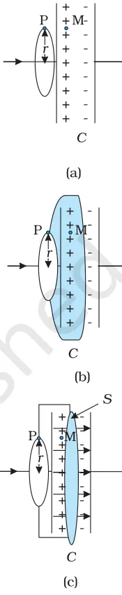
What it is: Displacement current is not a flow of charges but a term introduced by Maxwell to describe the effect of a time-varying electric field in producing a magnetic field. It completes Ampère's law so that the law holds for time-dependent situations (for example, inside the gap of a charging capacitor).

Why it was needed: Ampère's law in its original form (∮B·dl = μ0 I_enclosed) fails for cases like a charging capacitor if one chooses different surfaces bounded by the same loop (one surface cuts the wire, the other passes between the capacitor plates). Maxwell added the displacement-current term to restore consistency and to ensure charge conservation (continuity equation).

Definition: The displacement current density J_d in vacuum is

J_d = ε0 ∂E/∂t

More generally, in a medium with permittivity ε:

J_d = ε ∂E/∂t

Ampère–Maxwell law (integral form):

∮B·dl = μ0 I_enclosed + μ0 ε0 dΦ_E/dt

Here dΦ_E/dt is the rate of change of electric flux through the chosen surface and μ0 ε0 dΦ_E/dt represents the displacement current (in units of ampere).

Key physical example — charging capacitor:

• For a parallel-plate capacitor with plate area A and plate separation small compared to plate dimensions, the electric field between plates is E = Q/(ε0 A).
• Differentiate: ∂E/∂t = (1/(ε0 A)) dQ/dt = I/(ε0 A), where I = dQ/dt is the conduction current in the wire.
• Displacement current through the gap: I_d = ε0 A ∂E/∂t = I. Thus the displacement current equals the conduction current, and the magnetic field produced in the gap is the same as that produced by the wire current.

Mathematical consistency: In differential form the law is

∇×B = μ0 J + μ0 ε0 ∂E/∂t.

Taking divergence of both sides gives 0 = μ0(∇·J + ∂ρ/∂t), which is equivalent to the continuity equation ∇·J + ∂ρ/∂t = 0, so charge conservation is satisfied.

Role in electromagnetic waves: The displacement-current term couples time-varying electric fields to magnetic fields and — together with Faraday's law — leads to the wave equations

∇²E = μ0 ε0 ∂²E/∂t² and ∇²B = μ0 ε0 ∂²B/∂t²,

showing that time-varying fields propagate as electromagnetic waves with speed c = 1/√(μ0 ε0).

Units: J_d has SI units A·m⁻² (current density); I_d has units A (ampere).

What it states
The equation of continuity is the mathematical expression of local charge conservation. In differential form it is written as

∂ρ/∂t + ∇·J = 0

Here ρ(r,t) is the charge density and J(r,t) is the current density. It means that the rate of decrease of charge inside a small volume equals the net outward current flux through the surface of that volume.

Integral form
For a fixed volume V with surface S, the integral form is

d/dt ∫_V ρ dV + ∮_S J·dA = 0

This says the time rate of change of total charge in V plus the outward current through S is zero.

Derivation and connection to Maxwell's equations
Take the divergence of the Ampère–Maxwell law: ∇×B = μ0(J + ∂D/∂t). Since ∇·(∇×B)=0, we get 0 = μ0(∇·J + ∂/∂t ∇·D). Using Gauss’s law ∇·D = ρ, we obtain the continuity equation ∂ρ/∂t + ∇·J = 0. This shows charge conservation is built into Maxwell’s equations when the displacement current term (∂D/∂t) is included.

Physical meaning and importance
The equation enforces local conservation of electric charge: charge cannot suddenly appear or disappear at a point. It also motivated the displacement current term: in a charging capacitor there is no conduction current in the dielectric gap, yet the magnetic field behaves as if a current flows — the changing electric displacement (∂D/∂t) provides the required "displacement current" so the continuity equation remains valid.

Overview: Electromagnetic waves are time-varying electric and magnetic fields that propagate through space. Their behaviour follows from Maxwell's equations. In free space (no charges, no currents) these equations lead directly to a wave equation for both the electric field E and the magnetic field B, showing that they propagate with speed c = 1/sqrt(mu0 epsilon0).

Maxwell's equations in free space (differential form):

∇·E = 0

∇·B = 0

∇×E = −∂B/∂t

∇×B = μ0 ε0 ∂E/∂t

Derivation (for E):

1. Take the curl of Faraday's law: ∇×(∇×E) = −∂/∂t (∇×B).

2. Substitute ∇×B from Maxwell: −∂/∂t (μ0 ε0 ∂E/∂t) = −μ0 ε0 ∂^2 E/∂t^2.

3. Use the vector identity ∇×(∇×E) = ∇(∇·E) − ∇^2 E. In free space ∇·E = 0, so ∇×(∇×E) = −∇^2 E.

4. Equate both sides: −∇^2 E = −μ0 ε0 ∂^2 E/∂t^2.

5. Cancel negatives to obtain the wave equation for E:

∇^2 E = μ0 ε0 ∂^2 E/∂t^2

Similarly for B: By the same steps (take curl of ∇×B = μ0 ε0 ∂E/∂t and use ∇·B = 0) you get

∇^2 B = μ0 ε0 ∂^2 B/∂t^2

Wave speed: These are standard wave equations with speed v given by

v = 1 / sqrt(μ0 ε0)

In vacuum v = c ≈ 3.00 × 10⁸ m/s.

Plane-wave solution and properties:

A plane wave traveling in direction k̂ can be written as

E(r,t) = E0 cos(k·r − ωt + φ)

with the dispersion relation

ω / k = v = 1 / sqrt(μ0 ε0)

Fields are transverse: k·E = 0 and k·B = 0. B is related to E by

B = (1/v) k̂ × E

and the amplitudes satisfy B0 = E0 / v.

Energy and power flow:

Poynting vector gives instantaneous energy flux density:

S = (1/μ0) E × B

For a plane wave the average intensity is

<S> = (E0^2) / (2 μ0 v)

The time-averaged energy density (electric + magnetic) is

<u> = ε0 E0^2 / 2

Transverse nature and polarization: Since E and B are perpendicular to direction of propagation, electromagnetic waves can be polarized (direction of E vector). Polarization is an important practical property used in antennas, sunglasses, LCDs, etc.

Summary: Starting from Maxwell's equations in free space and using vector identities, one obtains wave equations for E and B showing that time-varying electromagnetic fields propagate as transverse waves at speed c = 1/sqrt(mu0 epsilon0). These waves carry energy described by the Poynting vector.

Definition. A plane electromagnetic (EM) wave is a solution of Maxwell's equations in which the electric field E and magnetic field B depend only on the phase (k·r − ωt). Wavefronts (surfaces of constant phase) are planes perpendicular to the propagation vector k.

Maxwell's equations in free space (no charges, no currents) lead to the wave equations:

• ∇·E = 0, ∇·B = 0
• ∇×E = −∂B/∂t
• ∇×B = μ0ε0 ∂E/∂t

Taking the curl of ∇×E and using the other relations gives the vector wave equations

• ∇²E = μ0ε0 ∂²E/∂t²
• ∇²B = μ0ε0 ∂²B/∂t²

These equations admit plane-wave solutions of the harmonic form (real form):

• E(r,t) = E0 cos(k·r − ωt + φ)
• B(r,t) = B0 cos(k·r − ωt + φ')

Dispersion relation and speed. For non-dispersive free space, ω and k satisfy

• ω = c |k|, where c = 1 / √(μ0 ε0) (speed of light in vacuum)

Transverse nature and field relation. For plane waves in free space:

• E · k = 0 and B · k = 0 (both fields are transverse to propagation)
• E, B and k are mutually perpendicular and form a right-handed triad
• Fields are in phase for the simple plane harmonic wave. The amplitude relation is |B0| = |E0|/c
• Vector relation: B = (1/c) k̂ × E (for a wave with k̂ = k/|k|)

Complex form (convenient for calculations). E(r,t) = Re{E0 e^{i(k·r − ωt)}}, similarly for B. This simplifies superposition and polarization analysis.

Energy and power flow. Instantaneous Poynting vector S = (1/μ0)(E × B). For a harmonic plane wave the time-averaged intensity (power per unit area) is

• <S> = (1/2) ε0 c E0^2 = (1/2) (E0^2/μ0 c)
• Energy density u = (ε0 E^2/2 + B^2/(2μ0)); for a plane wave average <u> = ε0 E0^2/2

Polarization. Characterizes direction and time-behavior of E at a fixed point:

• Linear polarization: E oscillates in a fixed direction.
• Circular polarization: two orthogonal equal-amplitude components with 90° phase difference → tip of E traces a circle.
• Elliptical polarization: general case → tip of E traces an ellipse.

Solutions summary. The complete set of plane-wave solutions in free space are E(r,t) = Re{E0 e^{i(k·r − ωt)}} with k·E0 = 0 and ω = c|k|; B obtained from B = (1/ω) k × E or B = (1/c) k̂ × E. Linear combinations (superposition) give more general waveforms and polarization states.

Important physical points to remember:

• Plane waves are idealizations — good approximations locally when wavefronts are nearly planar (far from sources).
• In vacuum phase and group velocities equal c; in dispersive media they may differ.
• Boundary conditions at interfaces and polarization determine reflection/refraction (Fresnel relations) but are beyond the basic plane-wave solution.

What it means: An electromagnetic (EM) wave is transverse because its electric field (E) and magnetic field (B) vectors oscillate in directions perpendicular to the direction of propagation (wavevector k), and they are also perpendicular to each other. This perpendicular arrangement allows EM waves to be polarized.

Why — from Maxwell's equations (in free space):

• ∇·E = 0 and ∇·B = 0 show there are no longitudinal (parallel-to-k) field components for free-space plane waves.
• ∇×E = −∂B/∂t and ∇×B = μ0ε0 ∂E/∂t lead to the wave equations for each field: ∇²E = μ0ε0 ∂²E/∂t² and ∇²B = μ0ε0 ∂²B/∂t², admitting transverse plane-wave solutions.

Plane-wave example (propagation along +x):

E(x,t) = E0 ŷ cos(kx − ωt)
B(x,t) = B0 ẑ cos(kx − ωt)

Here E is along y, B along z, propagation along x. For such a solution ω/k = c = 1/√(μ0ε0), and B0 = E0/c. Thus E ⟂ B ⟂ k and E, B oscillate in phase.

Energy and direction: The energy flux (Poynting vector) is S = (1/μ0) E × B, which points in the propagation direction k, consistent with E × B giving the direction of travel.

Consequences: Because the fields are transverse, EM waves can be polarized (linear, circular, elliptical). Longitudinal electromagnetic waves in free space do not exist for the simple solutions of Maxwell's equations (exceptions occur in guided media or plasmas where boundary/medium effects permit longitudinal components).

Experimental evidence (brief): Polarizing filters block light polarized in one direction, and dipole antennas emit/receive strong fields only when oriented with the wave's E-field — both show the transverse character.

Overview
In an electromagnetic (EM) wave (Class 12 CBSE), the electric field E and magnetic field B are intrinsically linked. They are perpendicular to each other and to the direction of propagation, have equal phase, and their magnitudes are related by the wave speed. These properties follow from Maxwell's equations.

Plane EM wave (simple form)
For a plane EM wave traveling in the +x direction one can write (choice of axes):

E(x,t) = E0 sin(kx - ωt) ŷ
B(x,t) = B0 sin(kx - ωt) ẑ
k = wave number, ω = angular frequency

Here E is along y, B is along z, and the wave vector k (propagation) is along x: E ⟂ B ⟂ k. The sinusoidal factors are identical, so E and B oscillate in phase (peaks and zeros occur at the same points in space and time).

Direction (right-hand rule)
The direction of propagation is given by E × B. For the example above ŷ × ẑ = +ˆx (right-hand rule).

Relation of magnitudes
In vacuum (or a non-dispersive homogeneous medium) the amplitudes satisfy

E0 = c B0   (in vacuum)

More generally in a medium with permittivity ε and permeability μ the wave speed v = 1/√(με) and

E0 = v B0

These relations come from Maxwell's curl equations and the wave equation.

Energy and power
Electric and magnetic energy densities are equal at every point for a plane EM wave:

u_E = (1/2) ε E^2,   u_B = (1/2μ) B^2  ⇒  u_E = u_B

Total energy density u = u_E + u_B = ε E^2 = B^2/μ. The Poynting vector gives power flow (energy flux density):

S = (1/μ) E × B

For a sinusoidal wave the average intensity is ⟨S⟩ = (1/2μ) E0 B0 = (1/2) ε c E0^2.

Why E = cB? (Sketch)
From Maxwell: ∇×E = −∂B/∂t and ∇×B = μ0 ε0 ∂E/∂t. For a plane wave these give relations between field amplitudes and the wave speed c = 1/√(μ0 ε0). Combining gives E0/B0 = 1/√(μ0 ε0) = c.

Key points to remember

• E, B and propagation direction are mutually perpendicular.
• E and B are in phase (for a plane wave in free space).
• Magnitude relation: E0 = c B0 (vacuum) or E0 = v B0 (medium).
• Energy densities of electric and magnetic fields are equal; Poynting vector gives direction and rate of energy transport.

Overview
Electromagnetic (EM) waves are time-varying electric and magnetic fields that propagate through space. Maxwell's equations predict that these fields satisfy a wave equation and travel with a definite speed. In vacuum this speed is the speed of light, c, a universal constant.

Derivation (outline)
From Maxwell's equations in free space (no charges, no currents):

• ∇ · E = 0, ∇ · B = 0
• ∇ × E = −∂B/∂t
• ∇ × B = μ0ε0 ∂E/∂t

Take the curl of Faraday's law: ∇ × (∇ × E) = −∂/∂t (∇ × B). Using vector identity ∇ × (∇ × E) = ∇(∇·E) − ∇²E and ∇·E = 0 gives −∇²E = −μ0ε0 ∂²E/∂t². Rearranged, this is the wave equation

∇²E = μ0 ε0 ∂²E/∂t²,

which is a standard wave equation with wave speed

c = 1/√(μ0 ε0).

Numerical value
Using μ0 = 4π × 10⁻⁷ H·m⁻¹ and ε0 ≈ 8.854187817×10⁻¹² F·m⁻¹,

c ≈ 2.998 × 10^8 m/s ≈ 3.00 × 10^8 m/s.

This is the speed of all electromagnetic radiation (radio, microwaves, visible light, X‑rays, gamma rays) in vacuum.

Fields relation
In a plane EM wave in free space, E, B and the direction of propagation are mutually perpendicular, and their magnitudes are related by

|E| = c |B|.

Energy density u and Poynting vector S are given by

u = (ε0 E^2 + B^2/μ0)/2,   S = (1/μ0) E × B,

showing how energy and energy flux travel with the wave.

Speed in a material medium
In a linear, homogeneous, isotropic medium with permeability μ and permittivity ε,

v = 1/√(μ ε).

Define relative permittivity εr = ε/ε0 and relative permeability μr = μ/μ0, then

v = c / √(εr μr).

The refractive index n is n = c/v = √(εr μr). For most optical materials μr ≈ 1 so n ≈ √εr and v ≈ c/n.

Frequency dependence (dispersion)
In real media ε (and sometimes μ) depend on frequency, so v depends on frequency. This leads to phase velocity v_p = ω/k and group velocity v_g = dω/dk. In dispersive media v_p ≠ v_g; information and energy travel with v_g (subject to causality constraints).

Conductors and attenuation
In conductors, EM waves are strongly attenuated and penetrate only a short distance (skin depth) given approximately by

δ = √(2 / (ω μ σ)),

where σ is conductivity and ω angular frequency. In good conductors waves are rapidly damped and do not propagate freely as in dielectrics.

Summary
The universal vacuum speed c = 1/√(μ0 ε0) ≈ 3×10^8 m/s is the propagation speed of electromagnetic waves in vacuum. In materials the speed is reduced by the medium's permittivity and permeability and can vary with frequency (dispersion).

Definition: Energy density of an electromagnetic (EM) wave is the energy stored per unit volume in the electric and magnetic fields that constitute the wave.

Electric and magnetic contributions: At any point the instantaneous energy density has two parts: the electric part u_E and the magnetic part u_B, where u_E = 1/2 ε₀ E² and u_B = 1/(2μ₀) B². These come from the energy stored in the electric field and magnetic field respectively.

Plane EM wave in vacuum: For a plane electromagnetic wave in vacuum E and B are perpendicular and related by B = E/c. Using c² = 1/(ε₀μ₀) one finds u_E = u_B at every instant, so the total instantaneous energy density is u = u_E + u_B = ε₀ E² = B² / μ₀. If the wave has amplitude E₀ and E(t) = E₀ cos(ωt – kx), then u(t) = ε₀ E₀² cos²(ωt – kx).

Time-average (over a cycle): For a sinusoidal wave the time-averaged energy density is <u> = ε₀ E₀²/2 = ε₀ E_rms² = B_rms² / μ₀. This is the quantity usually used when relating energy to measurable power flux.

Relation to intensity and Poynting vector: The instantaneous energy flux (power per unit area) is given by the Poynting vector S = (1/μ₀) E × B. For a plane wave its magnitude is S = (1/μ₀) EB and the time-average intensity I is <S> = I = c <u>. Thus intensity = (energy density) × (speed of propagation).

Physical meaning and consequences: Energy carried by EM waves can be absorbed and transferred to matter (heating, photoelectric effect, mechanical forces). Radiation pressure is directly related to energy density: for perfect absorption p = I/c = <u> and for perfect reflection p = 2I/c = 2<u>. Energy densities in common situations are typically very small (e.g. sunlight near Earth corresponds to microjoules per cubic metre).

What it is: The Poynting vector describes the rate and direction of electromagnetic energy flow. For electromagnetic fields E and B (in SI units) the instantaneous Poynting vector is defined as

S = (1/μ0) E × B

Here μ0 is the permeability of free space. The vector S gives the power (energy per unit time) crossing a unit area; its SI unit is watt per square metre (W m^-2). For general materials one often uses the equivalent form S = E × H, where H = B/μ.

Poynting theorem (energy conservation for EM fields): In differential form the theorem is

∂u/∂t + ∇·S = -J·E

where u is the electromagnetic energy density and J·E is the work done per unit volume per unit time on charges. The energy density is

u = 1/2 (ε0 E^2 + (1/μ0) B^2)

This equation means: the decrease of field energy in a volume plus the net outward electromagnetic energy flux (given by S) equals the energy delivered to charges inside the volume.

For a plane electromagnetic wave in vacuum: E, B and the propagation direction are mutually perpendicular and E and B are in phase. The fields satisfy E = c B. The instantaneous magnitude of S becomes

|S| = (1/μ0) E B = ε0 c E^2 = (1/μ0) c B^2

The time-averaged energy flux (intensity) for harmonic fields E(t) = E0 cos(ωt) is

Additional useful relations: intrinsic impedance of free space Z0 = sqrt(μ0/ε0) ≈ 377 ohm gives . Radiation pressure exerted on a surface is related to S: for complete absorption p = <S>/c, for perfect reflection p = 2 <S>/c.

Physical meaning and sign: The direction of S is the direction in which electromagnetic energy is transported. In waves it points along the propagation direction. Instantaneous S may oscillate, but its time average for a travelling wave is positive in the propagation direction.

What it states (simple): The Poynting theorem expresses conservation of electromagnetic (EM) energy. It relates the rate of change of EM energy in a region to the net EM energy flow out of that region and the work done on charges inside it.

Key quantities:

• Poynting vector S = (1/μ0) E × B. It gives the instantaneous power flow (energy per unit area per unit time) and points in the direction of energy flow.
• EM energy density u = 1/2 (ε0 E^2 + B^2/μ0). This is the energy stored per unit volume in the fields.

Differential form (local conservation):

∂u/∂t + ∇·S = −J·E

Interpretation: the increase of field energy density u in a small volume plus the net outward flux of EM energy (∇·S) equals the negative of the work done per unit volume per unit time on charges (J·E). If J·E>0, fields do work on charges (field energy decreases).

Integral form (global conservation):

∂/∂t ∫_V u dV + ∮_S S·dA = − ∫_V J·E dV

Interpretation: rate of decrease of total EM energy in volume V plus net outflow of EM power through surface S equals the power delivered to charges in V.

Plane wave example (useful relations): For a plane EM wave in vacuum, E and B are perpendicular and B = E/c. Instantaneous S = (1/μ0) E × B has magnitude S(t) = (E^2)/(μ0 c) sin^2(kx−ωt). The time-averaged intensity (average Poynting magnitude) is ⟨S⟩ = (E0^2)/(2 μ0 c) = (1/2) ε0 c E0^2.

Physical meaning: S tells you how much electromagnetic energy crosses a unit area per second and in what direction. The theorem shows that EM energy can be transported by fields, stored in fields, and converted to mechanical or thermal energy by doing work on charges (J·E term).

When useful in Class 12 problems: calculating intensity of EM wave, power transmitted along cables or into a resistor (by integrating S over a surface), and understanding radiation pressure and energy transfer in devices like antennas, microwave ovens and solar panels.

Overview
Electromagnetic (EM) waves carry energy and momentum. When EM radiation strikes a surface, transfer of momentum produces a mechanical force per unit area called radiation pressure. Radiation pressure arises both from the wave nature (Poynting flux) and from the photon picture (each photon carries momentum).

Energy, Poynting vector and momentum density
For an electromagnetic field in vacuum the instantaneous energy density is u = (ε0E^2 + B^2/μ0)/2. The Poynting vector S = (1/μ0)(E × B) gives the energy flux (power per unit area). For a plane wave in vacuum |E| = c|B| and the time-averaged intensity (power per unit area) is I = <S> = u c.

The electromagnetic momentum density g (momentum per unit volume) is related to energy density by

g = u/c = S/c^2.

Photon picture
Each photon of frequency ν has energy E = hν and momentum p = E/c = hν/c. A flux of photons incident on a surface transfers momentum when photons are absorbed or reflected, producing radiation pressure.

Radiation pressure on a surface (normal incidence)
- Perfectly absorbing surface (normal incidence): the incident energy flux I delivers momentum at rate I/c per unit area, so pressure P = I/c.
- Perfectly reflecting surface (normal incidence): the normal component of photon momentum is reversed, doubling the momentum change, so P = 2I/c.

General (angle and reflectivity)
For a beam incident at angle θ to the surface normal the effective incident power on area A is I A cosθ. The normal component of momentum transfer introduces a cosθ factor, giving a cos^2θ dependence. If a fraction R of the incident energy is reflected and a fraction A is absorbed (R + A + T = 1), commonly used forms are:

• For negligible transmission (T ≈ 0): P = (I/c)(1 + R) cos^2θ. (R = 0 → absorbing: P = I cos^2θ / c; R = 1 → reflecting: P = 2I cos^2θ / c.)
• More generally, considering reflected and transmitted momentum components, one can write P = (I/c)(2R + A) cos^2θ, using A = absorbed fraction.

Physical interpretation & magnitudes
Radiation pressure is very small for ordinary light intensities because c is large: for sunlight (I ≈ 1.36 kW/m2 at Earth) the pressure on a perfect absorber is ≈ 4.5 × 10^-6 N/m2, and ≈ 9 × 10^-6 N/m2 for a perfect reflector. Nevertheless it is important in astrophysics (stellar winds, dust dynamics) and in precise laboratory setups (optical tweezers, laser cooling, photon rockets, solar sails).

Limitations / notes
- Devices like the Crookes radiometer are often cited in popular accounts as demonstrating radiation pressure; in fact the dominant effect there is thermal gas effects, not direct radiation pressure.
- The above formulas assume plane waves and classical specular reflection/absorption; scattering, diffuse reflection and material response can modify results.

Summary: When electromagnetic waves travel in a conducting medium (conductivity σ > 0), conduction current (σE) appears in Maxwell's equations. That modifies the wave equation: waves are attenuated (damped) as they propagate, have a complex propagation constant, and penetrate only a finite depth (skin depth).

Governing equation: From Maxwell's equations (assuming homogeneous, isotropic medium with permittivity ε, permeability μ, conductivity σ) the electric field satisfies

∇²E = μ ε ∂²E/∂t² + μ σ ∂E/∂t.

For a plane wave E(z,t) = E₀ e^{i(βz − ωt)} e^{-αz}, combine terms to get the complex propagation constant γ = α + iβ:

γ² = μ ε ω² + i μ σ ω = μ ω (ε ω + i σ).

Thus the field inside the conductor behaves as

E(z,t) = E₀ e^{-α z} e^{i(β z − ω t)}.

Key physical consequences:

• Attenuation: amplitude decays exponentially with distance inside conductor; α is the attenuation constant.
• Phase advance: β is the phase constant; in conductors α and β are generally comparable.
• Skin effect: currents and fields are confined to a thin surface layer of thickness called skin depth δ = 1/α for good conductors.
• Energy dissipation: the wave energy is dissipated as Joule heat (power density = σ E²).
• Limits: Two useful regimes—"good conductor" (σ >> ωε) and "poor conductor" (σ << ωε)—give simple approximations for α, β and impedance.

Good conductor (σ >> ωε) – metals at typical RF and below:

• Propagation constant ≈ (1 + i) sqrt(π f μ σ) (since ω = 2π f), so α ≈ β ≈ sqrt(π f μ σ).
• Skin depth δ = 1/α = sqrt(2/(μ σ ω)) = sqrt(1/(π f μ σ)).
• Wave impedance Z ≈ (1 + i) sqrt(ω μ /(2 σ)) (a small, complex number); E and H are nearly in phase but with a 45° phase shift between them.

Poor conductor (σ << ωε) – weakly conducting dielectrics:

• α ≈ (σ/2) sqrt(μ/ε) (small), β ≈ ω sqrt(μ ε) (≈ propagation in dielectric).
• Conductive losses are small; wave propagates with little attenuation but some energy is absorbed gradually.

Boundary and reflection behavior: A good conductor strongly reflects incident EM waves because they cannot penetrate deeply. The reflected wave acquires a phase (near −1 for an ideal conductor). For finite conductivity, a thin layer (skin depth) absorbs the field.

Typical magnitudes (examples): For copper (σ ≈ 5.8×10⁷ S/m, μ≈μ₀): at 60 Hz δ ≈ 8.5 mm; at 1 MHz δ ≈ 66 μm. Thus high-frequency currents concentrate near the surface: the skin effect.

Energy balance: Poynting vector into the conductor is dissipated as Joule heating. Inside conductor average power dissipated per unit volume = (1/2) σ |E|².

Takeaway: Conductivity converts propagating electromagnetic energy into heat and drastically reduces penetration depth. This underlies shielding, wave absorption in sea water, skin effect in wires, induction heating, and limits transmission in conductive environments.

Skin effect is the tendency of alternating current (AC) to concentrate near the surface of a conductor, rather than being uniformly distributed across its cross-section. This happens because the time-varying magnetic field produced by the AC induces eddy currents inside the conductor that oppose the main current (Lenz's law), forcing the net current density to decrease rapidly with depth from the surface.

Physical picture: For an AC of angular frequency ω, the magnetic field inside the conductor changes with time. These changing fields induce secondary currents that oppose the interior current flow, so the amplitude of current density J (and the associated electric and magnetic fields) decays exponentially with depth x into the conductor.

Mathematical description: For a plane wave or uniform surface current on a large conductor, the current density as a function of depth is
J(x) = J(0) e^{-x/δ} e^{-i x/δ}
so the magnitude |J(x)| = |J(0)| e^{-x/δ}. The factor e^{-i x/δ} shows a phase lag that increases with depth (45° phase change per skin depth in a good conductor).

Skin depth (δ): The skin depth is the characteristic depth at which the amplitude of the current density (or field) falls to 1/e (≈37%) of its surface value. For a linear, isotropic conductor with conductivity σ and permeability μ, and angular frequency ω = 2πf,

δ = sqrt{2 / (ω μ σ)} = sqrt{1 / (π f μ σ)}

For a good conductor (σ >> ωε), the complex propagation constant inside the conductor is γ = (1 + i)/δ, so the attenuation constant α and phase constant β are equal: α = β = 1/δ. Power density (∝ |J|^2) therefore decays as e^{-2x/δ}, i.e. to about 13.5% at x = δ.

Consequences:

• The effective AC resistance of a conductor increases with frequency because the current is confined to a thinner surface layer (smaller effective cross-sectional area).
• At high frequencies the conductor behaves as if current flows only in a thin surface layer; this increases I^2R losses and heating.
• The skin depth decreases with increasing frequency and with increasing permeability and conductivity (δ ∝ 1/√(f μ σ)).

Typical values (copper, μ ≈ μ0 = 4π×10^-7 H/m, σ ≈ 5.8×10^7 S/m):

• At f = 50 Hz, δ ≈ 9.4 mm (so skin effect is small for thin wires but may matter for very large conductors or busbars).
• At f = 1 MHz, δ ≈ 66 μm (current confined to a very thin surface layer).

Mitigation: Use stranded insulated wires (Litz wire) for high-frequency windings, use tubular conductors, silver-plating, or use thin conductive coatings; design transformers and conductors to reduce eddy currents and losses.

Overview
When an electromagnetic plane wave travels through a material medium (characterized by permittivity ε, permeability μ and conductivity σ), its amplitude may decay and its phase change with distance. The wave is described by a complex propagation constant γ = α + iβ where α is the attenuation constant (Np/m) and β is the phase constant (rad/m).

Wave form in a medium
For a wave propagating in +z direction the field can be written as
E(z,t) = E₀ e^−αz cos(ωt − βz).

General expression for the propagation constant
From Maxwell's equations (plane-wave ansatz) one obtains

    γ = α + iβ = ω sqrt(με) sqrt(1 + i σ/(ωε)).
Introduce the loss parameter m = σ/(ωε). Writing the complex square-root gives closed forms for α and β:

    α = ω sqrt(με) sqrt((sqrt(1 + m^2) - 1)/2),

    β = ω sqrt(με) sqrt((sqrt(1 + m^2) + 1)/2).

Special cases
1) Lossless dielectric (σ = 0): m = 0, so α = 0 and β = ω sqrt(με). The wave does not attenuate and travels with phase velocity v_p = 1/sqrt(με) = c/n.
2) Good conductor (σ >> ωε): m >> 1 and α ≈ β ≈ sqrt(ωμσ/2). Thus fields decay very rapidly inside conductors (skin effect).

Skin depth
The skin depth δ (the distance where amplitude falls to 1/e) is δ = 1/α. For a good conductor approximately
    δ ≈ sqrt(2/(ωμ&sigma)).

Phase velocity and dispersion
Phase velocity is defined by
    v_p = ω/β.
Because β generally depends on frequency (ω), v_p is frequency dependent (dispersion). In some media or structures v_p can exceed c; this does not violate relativity because signal and energy transport are governed by group velocity and causality.

Complex refractive index
It is common to introduce a complex refractive index ñ = n - iκ with the relations
    β = (ω/c) n,    α = (ω/c) κ.
Thus attenuation is encoded in the extinction coefficient κ.

Physical consequences
Attenuation causes exponential amplitude reduction and frequency-dependent phase shift, leading to signal weakening and pulse distortion. In conductors the skin effect concentrates currents near the surface. In communications and optics, choosing frequency and material to minimize unwanted α is essential.

Definition: Polarization of an electromagnetic (EM) wave describes the time-varying direction of the electric field vector E at a fixed point in space. Because EM waves in free space are transverse, the E vector lies in the plane perpendicular to the direction of propagation. Polarization specifies how that vector rotates or oscillates with time.

Physical idea (Class 12 level): For a wave traveling in the +z direction the electric field can be written as two perpendicular components in the x and y directions:

E_x = E_0x cos(kz - ωt)
E_y = E_0y cos(kz - ωt + δ)

Different choices of amplitudes E_0x, E_0y and phase difference δ give different polarizations:

• Linear polarization: δ = 0 or π. E lies along a fixed line (e.g., x or y or any fixed direction in the x–y plane).
• Circular polarization: E_0x = E_0y and δ = ±π/2. The tip of E traces a circle; handedness (right/left) depends on the sign of δ.
• Elliptical polarization: The general case: unequal amplitudes or arbitrary δ. The tip of E traces an ellipse.

How polarization is produced:

• Polarizing filters (Polaroids): absorb one component of E, transmitting mainly one linear polarization.
• Reflection at a dielectric surface (Brewster's angle): light reflected at Brewster's angle is fully linearly polarized with E perpendicular to the plane of incidence.
• Scattering (Rayleigh): sunlight scattered by the atmosphere becomes partially polarized (reason for polarized sky patterns).
• Optical devices: quarter-wave plates and half-wave plates introduce controlled phase differences to convert linear ↔ circular or rotate linear polarization.

How polarization is analyzed: Using a second polarizer (analyzer). For ideal linear polarizers, transmitted intensity follows Malus' law (see formulas). For devices like wave plates, a phase delay δ is introduced between components to change polarization type.

Important points for Class 12: Polarization is a property only of transverse waves (so not defined for longitudinal waves). Polarization does not affect the frequency ω or wave number k (only amplitudes and relative phase). Many practical devices exploit polarization for reducing glare, controlling light in displays, and measuring stresses in materials (photoelasticity).

What are boundary conditions?
Boundary conditions at an interface are the rules that relate the electric and magnetic fields immediately on one side of a surface to the fields immediately on the other side. They come directly from Maxwell's equations (Gauss's laws, Faraday's law and Ampère–Maxwell law) and tell how field components change (or remain continuous) when crossing a boundary between two materials.

How they are obtained (briefly)
Take very small Gaussian surfaces and rectangular loops that straddle the interface and apply the integral forms of Maxwell's equations. Let n̂ be a unit vector normal from medium 1 into medium 2.

Basic boundary conditions (general form)

• From Faraday's law (no infinite rate of change): the tangential component of electric field is continuous across the interface:
  n̂ × (E1 − E2) = 0 → E1_tangential = E2_tangential
• From Gauss's law for electricity: the normal components of electric displacement D differ by the surface free charge density σs:
  n̂ · (D2 − D1) = σs
• From Gauss's law for magnetism: the normal component of magnetic flux density is continuous (no magnetic monopoles):
  n̂ · (B2 − B1) = 0 → B1_normal = B2_normal
• From Ampère–Maxwell law: the tangential components of magnetic field H jump by any surface current density Js:
  n̂ × (H2 − H1) = Js → H2_tangential − H1_tangential = n̂ × Js

Common simplified cases

• If there are no free surface charges (σs = 0) and no surface currents (Js = 0) — typical for two dielectrics: tangential E and tangential H are continuous; normal D and normal B are continuous.
• Perfect conductor boundary: inside a perfect conductor E = 0 and B = 0 (steady state). At its surface, tangential E just outside = 0 and H_tangential = surface current density. Normal component of B inside = 0.

Physical meaning and consequences
Continuity of tangential E implies that an oscillating electric field cannot have a sudden tangential jump at the interface — this underlies Snell's law and the Fresnel relations for reflection and transmission. Continuity/discontinuity of D and B relate to how charges or magnetic flux are redistributed at surfaces. These boundary conditions are the starting point for deriving reflection coefficients, transmission coefficients, Brewster angle, and behavior in waveguides and optical coatings.

How to use them (sketch)
To find reflected and transmitted fields for a plane wave incident on a plane interface: write incident, reflected and transmitted field phasors; apply the boundary conditions to tangential E and H at the interface (or both components for s- and p-polarizations). Solve the linear equations to get reflection and transmission amplitudes (Fresnel coefficients).

Note: For Class 12 level the key idea is: use small loops and pillboxes to translate Maxwell's equations into simple continuity conditions for tangential and normal components of E, D, H and B at boundaries.

What is the electromagnetic spectrum?

The electromagnetic (EM) spectrum is the full range of electromagnetic waves arranged by wavelength (λ) or frequency (ν). All EM waves travel in vacuum with the same speed c ≈ 3.00 × 10⁸ m s⁻¹, are transverse (electric field E ⟂ magnetic field B ⟂ direction of propagation k), and carry energy and momentum. Different parts of the spectrum differ only by frequency/wavelength and hence photon energy; this gives them different physical effects and uses.

Key regions (approximate ranges)

• Radio waves: longest wavelengths — from about 10⁴ m down to ~1 m (frequencies ≈ 3 kHz to 300 MHz). Used for broadcasting and communication.
• Microwaves: λ ≈ 1 m to 1 mm (frequencies ≈ 300 MHz to 300 GHz). Used in radar, microwave ovens, satellite links.
• Infrared (IR): λ ≈ 1 mm to 700 nm. Thermal radiation, remote controls, night-vision.
• Visible: λ ≈ 700 nm (red) to 400 nm (violet). Light detectable by human eye; optics and imaging.
• Ultraviolet (UV): λ ≈ 400 nm to 10 nm. Causes fluorescence, sunburn; used for sterilization.
• X-rays: λ ≈ 10 nm to 0.01 nm. Medical imaging and crystallography.
• Gamma rays: shortest wavelengths: λ < 0.01 nm (very high frequency). Produced by nuclear transitions; used in cancer therapy and sterilization.

Physical principles

• Speed in vacuum: c = λν (same for all EM waves in vacuum).
• Photon energy: E = hν (h = Planck's constant ≈ 6.626×10⁻³⁴ J·s). Thus higher frequency → higher energy per photon.
• EM waves satisfy the wave equation (in vacuum): ∇²E = (1/c²) ∂²E/∂t² (and similarly for B).
• Interactions with matter depend on energy: radio/microwave/IR are generally non‑ionizing; UV, X‑rays and γ‑rays are ionizing and can damage biological tissue.

Applications and why different parts are used

• Radio & TV broadcasting: long wavelengths diffract around obstacles and propagate over long distances.
• Microwaves: excite molecular rotations (water) — basis for microwave heating; short wavelengths allow reasonably small antennas and directional transmission (radar, satellite).
• Infrared: thermal imaging and remote sensing — emitted by warm objects; fiber‑optic communication uses near‑IR where silica loss is low.
• Visible light: imaging, microscopy, optical fibers (visible and near‑IR), and illumination.
• Ultraviolet: sterilization (kills microbes), fluorescence for detection; also responsible for photochemical reactions in atmosphere and skin.
• X‑rays and γ‑rays: penetrate matter — useful for imaging internal structure (X‑rays) and for radiotherapy (γ‑rays).

Safety note: UV, X‑rays and gamma rays are ionizing; exposure must be controlled. Microwaves and strong IR can cause heating; long‑wavelength radio waves are generally low energy per photon and non‑ionizing but high power can heat tissue.

Overview
Electromagnetic waves are solutions of Maxwell's equations. To understand their form and properties you need several mathematical tools: vector calculus (divergence, curl, Laplacian), partial differential equations (wave equation and Helmholtz equation), complex exponentials (phasor notation), and boundary-condition methods. These tools let you derive the wave equation, obtain plane-wave solutions, relate electric and magnetic fields, and compute energy and power flow.

Essential mathematical steps (sketch)

• Start from Maxwell's equations in free space (vacuum):
  • div E = 0
  • div B = 0
  • curl E = −∂B/∂t
  • curl B = μ0 ε0 ∂E/∂t
• Take curl of curl of E and use the vector identity curl(curl E) = grad(div E) − ∇²E. With div E = 0 this gives the wave equation
  ∇²E − μ0 ε0 ∂²E/∂t² = 0
• Analogously for B: ∇²B − μ0 ε0 ∂²B/∂t² = 0. These are second-order linear PDEs whose general solutions are waves propagating at speed c = 1/√(μ0 ε0).
• Use the plane-wave ansatz (phasor form) E(r,t) = Re{E0 e^{i(k·r − ωt)}}. Substitute to obtain the dispersion relation k^2 = ω^2 μ0 ε0 and the transversality condition k·E0 = 0 (fields are perpendicular to propagation).
• From curl E = −∂B/∂t and the plane-wave form obtain B0 = (1/ω) k × E0, so E, B and k are mutually perpendicular and |E0| = c |B0|.

Other important mathematical concepts

• Phasors & complex notation: simplify time derivatives via factor iω and solve algebraic equations for amplitudes.
• Boundary conditions: continuity of tangential E and normal components of D etc., used for reflection and transmission at interfaces.
• Poynting vector and energy density: quantify power flow and stored energy using vector operations.
• Dispersion and group velocity: in dispersive media ω(k) is not linear; group velocity dω/dk determines pulse motion.

Why these tools matter
They let you predict wave speed, polarization, intensity, energy transport, reflection/transmission at surfaces, and behavior in media (conductors, dielectrics). These are the mathematical foundations behind radio, microwave, optical and many technological applications.