Overview
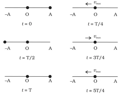
Introduction: Oscillations describe repetitive back-and-forth motion about an equilibrium position. This chapter introduces periodic motion and its simplest form — simple harmonic motion (SHM) — and shows how SHM models many physical systems (mass–spring, simple pendulum, atoms in solids, electrical oscillators). Importance: Understanding oscillations is foundational for waves, sound, optics and many engineering applications (clocks, seismology, suspension systems). The mathematical tools learned (differential equations, small-angle approximation, energy methods) are widely used across physics. Key themes: definition of periodic and oscillatory motion; distinguishing between general periodic motion and SHM; deriving the SHM differential equation; solutions and their physical interpretation (amplitude, angular frequency, phase); velocity and acceleration relationships; energy exchange between kinetic and potential forms; examples (mass–spring system and simple pendulum) and how their time periods depend on system parameters; graphical representation of displacement, velocity and acceleration; relation between SHM and uniform circular motion; small oscillations approximation and…
Learning Objectives
- Define periodic motion, oscillation, amplitude, period, frequency, angular frequency and phase, and state their SI units.
- Show that a particle with displacement x = A cos(ωt + φ) satisfies the simple harmonic motion (SHM) equation and identify A, ω and φ physically.
- Derive the differential equation d²x/dt² + ω²x = 0 for SHM from Hooke's law (restoring force ∝ displacement).
- Calculate instantaneous velocity and acceleration in SHM from x(t) and determine their phase relationships with displacement.
- Derive expressions for kinetic, potential and total energy in SHM and use them to show conservation of mechanical energy.
- Derive the time period of a mass–spring system (T = 2π√(m/k)) and apply it to solve numerical problems involving k, m, T and ω.
- Derive the time period of a simple pendulum for small oscillations (T = 2π√(l/g)) and apply it to compute g from experimental data.
- Apply SHM formulae to solve numerical problems on amplitude, period, frequency, phase constant, maximum speed and energy.
Topics in this chapter
13 topics · tap a topic title to jump straight to it.
Periodic and Oscillatory Motion
Oscillatory motion is motion in which a system moves back and forth about a stable equilibrium position. The position of the object repeatedly returns toward the equilibrium and then away, forming cycles.
Periodic motion is a special type of oscillatory motion that exactly repeats itself after a fixed time interval called the period (T). Mathematically, a motion x(t) is periodic if x(t + T) = x(t) for all t. Frequency (f) is the number of cycles per second: f = 1/T. Angular frequency (ω) relates to frequency by ω = 2πf = 2π/T.
Important terms: equilibrium (mean) position, amplitude (A) — maximum displacement from equilibrium, period (T), frequency (f), angular frequency (ω), and phase (φ) — which sets the initial condition of the motion.
Simple Harmonic Motion (SHM) is the important ideal case of oscillatory motion where the acceleration is directly proportional to the displacement from equilibrium and directed toward it: a = −ω2x. The displacement as a function of time for SHM is commonly written as
x(t) = A cos(ωt + φ) or x(t) = A sin(ωt + φ),
where A is amplitude and φ is the phase constant. Velocity and acceleration follow from time derivatives:
v(t) = dx/dt = −A ω sin(ωt + φ)
a(t) = d2x/dt2 = −A ω2 cos(ωt + φ) = −ω2 x(t).
Energy in SHM: kinetic and potential energies exchange periodically while the total mechanical energy stays constant for an ideal (undamped) oscillator. For a mass–spring SHM (spring constant k and mass m),
Etotal = 1/2 k A2 = 1/2 m ω2 A2,
Potential energy: U = 1/2 k x2. Kinetic energy: K = Etotal − U.
Common physical realizations and formulas: a mass on a spring is an SHM with ω = sqrt(k/m) and period T = 2π sqrt(m/k). A simple (small-angle) pendulum of length L has T = 2π sqrt(L/g) for small angular displacements (θ small). AC electrical signals are another example of periodic oscillations (voltage or current varying sinusoidally).
Notes: Real oscillations often include damping (amplitude decreases with time) or forcing (external periodic driving). These lead to more complex behavior (damped oscillations, driven resonance) but the basic definitions of periodicity and oscillation still apply.
- Mass attached to a spring oscillating horizontally or vertically (ideal SHM).
- Simple pendulum (small amplitude) swinging about equilibrium.
- Tuning fork vibrating to produce a musical note (nearly periodic).
- Quartz crystal oscillator in wristwatches (stable periodic oscillation).
- Alternating current (AC) voltage and current — sinusoidal periodic signals.
- Child on a swing (oscillatory; approximates SHM for small angles).
- Condition for periodic motion: x(t + T) = x(t)
- Frequency and period: f = 1/T
- Angular frequency: ω = 2πf = 2π/T
- SHM displacement: x(t) = A cos(ωt + φ) or x(t) = A sin(ωt + φ)
- Velocity: v(t) = −A ω sin(ωt + φ)
- Acceleration: a(t) = −ω² x(t) = −A ω² cos(ωt + φ)
Simple Harmonic Motion (SHM): Definition and Equation
Definition: Simple Harmonic Motion (SHM) is the periodic motion of a particle about a fixed equilibrium position, where the acceleration of the particle is directly proportional to its displacement from equilibrium and is always directed towards that equilibrium (restoring acceleration). Mathematically, this restoring acceleration satisfies a = -omega^2 x.
Equation of motion: For SHM the displacement x(t) from equilibrium satisfies the linear second-order differential equation
d2x/dt2 + ω2 x = 0,
where ω (angular frequency) is a constant that depends on the system. The general solution is
x(t) = A cos(ωt + φ),
where A is the amplitude (maximum displacement) and φ is the phase constant determined by initial conditions. From x(t) we get velocity and acceleration:
- v(t) = dx/dt = -A ω sin(ωt + φ)
- a(t) = d2x/dt2 = -A ω2 cos(ωt + φ) = -ω2 x(t)
Frequency and period: ω relates to the period T and frequency f by
- ω = 2π f = 2π/T
- T = 2π/ω , f = 1/T
Physical origin: SHM occurs when the net restoring force is proportional to and opposite in sign to displacement: F = -k x (Hooke's law). For a mass m on a spring, ω = sqrt(k/m) and the equation of motion becomes d2x/dt2 + (k/m) x = 0.
Energy in SHM: Energy oscillates between kinetic and potential forms while total mechanical energy remains constant (in ideal, undamped SHM):
- Potential energy U = 1/2 k x2
- Kinetic energy K = 1/2 m v2 = 1/2 m ω2 (A2 - x2)
- Total energy E = K + U = 1/2 k A2 = constant
Examples of systems with simple harmonic approximation: small oscillations of a simple pendulum (for small angle), mass-spring systems, small vibrations of molecules about equilibrium positions, and small oscillations of a floating object. Real systems may have damping and driving forces, which modify pure SHM.
- Mass-spring oscillator: A block of mass m attached to a spring with spring constant k oscillates with angular frequency ω = sqrt(k/m) and period T = 2π sqrt(m/k).
- Simple pendulum (small angles): A bob of length L oscillates with ω = sqrt(g/L) and period T = 2π sqrt(L/g) when the angular displacement is small (sin theta ≈ theta).
- Tuning fork or vibrating string: Small vibrations approximate SHM and produce nearly sinusoidal displacement and sound.
- Clock pendulum and seismometer: Use the regular periodicity of near-SHM for timekeeping and measuring ground motion.
- Equation of motion: d^2x/dt^2 + ω^2 x = 0
- General solution: x(t) = A cos(ω t + φ)
- Velocity: v(t) = -A ω sin(ω t + φ)
- Acceleration: a(t) = -ω^2 x(t)
- Angular frequency and period: ω = 2π f = 2π/T, T = 2π/ω, f = 1/T
- Mass-spring: ω = sqrt(k/m), T = 2π sqrt(m/k)
Mathematical Solution of SHM
Definition: Simple Harmonic Motion (SHM) is motion in which the acceleration of a particle is always proportional to its displacement from a fixed point (equilibrium) and is directed toward that point. Mathematically, a(t) = -ω² x(t).
Derivation from Hooke's law (mass-spring):
For a mass m attached to a spring of force constant k, the restoring force is F = -kx. Using Newton's 2nd law, m d2x/dt2 = -kx. Divide by m to get the standard differential equation of SHM:
d2x/dt2 + (k/m) x = 0
Define the angular frequency ω by ω = sqrt(k/m). Then the equation is
d2x/dt2 + ω2 x = 0
General solution:
Solving the differential equation (characteristic roots ±iω) gives the general solution
x(t) = C1 cos(ωt) + C2 sin(ωt)
This can be written in amplitude-phase form
x(t) = A cos(ωt + φ)
where A = sqrt(C12 + C22) and φ is the phase constant determined by initial conditions.
Initial conditions: If x(0) = x0 and v(0) = v0, then
x0 = A cos φ
v0 = -A ω sin φ
So φ can be found from tan φ = -v0/(ω x0) (when x0 ≠ 0) and A = sqrt(x02 + (v0/(ω))2).
Velocity and acceleration:
v(t) = dx/dt = -A ω sin(ωt + φ)
 a(t) = d2x/dt2 = -A ω2 cos(ωt + φ) = -ω2 x(t)
Note acceleration is proportional to -x and is 180° out of phase with displacement.
Period and frequency:
Period: T = 2π/ω
 Frequency: f = 1/T = ω/(2π)
Energy in SHM (for mass-spring):
Potential energy: U = 1/2 k x(t)2
Kinetic energy: K = 1/2 m v(t)2 = 1/2 m ω2 (A2 - x2)
Total energy (constant): E = K + U = 1/2 k A2
Physical meaning: SHM describes oscillatory systems near stable equilibrium where restoring force is linear in displacement. The motion is sinusoidal in time with fixed amplitude and frequency determined by system parameters (m, k or g, L for a pendulum).
- Mass attached to a spring (horizontal or vertical) — displacement obeys d²x/dt² + (k/m)x = 0.
- Simple pendulum for small angles (θ small): angular SHM with ω = sqrt(g/L).
- Tuning fork or vibrating string segments approximated as SHM of elements.
- Balance wheel in mechanical watches approximated by SHM.
- Small oscillations of molecules about equilibrium positions (approximate SHM).
- LC electrical circuit (analogy): charge q satisfies d²q/dt² + (1/LC) q = 0 — electrical SHM.
- Differential equation: d²x/dt² + ω² x = 0
- Angular frequency (spring): ω = sqrt(k/m)
- Angular frequency (small-angle pendulum): ω = sqrt(g/L)
- General solution: x(t) = C1 cos(ωt) + C2 sin(ωt) = A cos(ωt + φ)
- Velocity: v(t) = -A ω sin(ωt + φ)
- Acceleration: a(t) = -A ω² cos(ωt + φ) = -ω² x(t)
Kinematics of SHM
Simple Harmonic Motion (SHM) is the motion of a particle about an equilibrium position where the acceleration is always directed towards the equilibrium and is proportional to the displacement from it. If x(t) denotes displacement from equilibrium, the defining differential equation is m d2x/dt2 + kx = 0 (for a linear restoring force), or in standard form d2x/dt2 + ω2x = 0, where ω is the angular frequency.
General solution: The displacement as a function of time is x(t) = A cos(ωt + φ), where A is the amplitude and φ the phase constant determined by initial conditions. From this follows the velocity and acceleration:
v(t) = dx/dt = −A ω sin(ωt + φ),
a(t) = d2x/dt2 = −A ω2 cos(ωt + φ) = −ω2 x(t).
Key kinematic features:
- a = −ω2x: acceleration is proportional and opposite to displacement.
- Velocity is 90° (π/2) out of phase with displacement: when x is maximum, v = 0; when x = 0 (equilibrium), |v| is maximum.
- Acceleration is 180° (π) out of phase with displacement: when x is positive, acceleration is negative, and vice versa.
- Period and frequency: T = 2π/ω and f = 1/T. Angular frequency relates as ω = 2πf.
Connection with uniform circular motion: SHM can be obtained as the projection of uniform circular motion of radius A onto a diameter. The projection coordinate executes x(t) = A cos(ωt + φ), which gives the same time dependence and phase relations for v and a.
Initial conditions and phase: Given x(0) = x0 and v(0) = v0, amplitude A and phase φ satisfy x0 = A cos φ and v0 = −A ω sin φ, so A = sqrt(x02 + (v0/ω)2) and φ = arctan(−v0/(ω x0)) (choose correct quadrant).
Special cases: For a mass-spring system m d2x/dt2 + kx = 0, ω = sqrt(k/m). For a simple pendulum (small angles) ω = sqrt(g/L).
- Mass attached to a horizontal spring oscillating on a frictionless surface (mass–spring system): x(t) = A cos(ωt + φ) with ω = √(k/m).
- Simple pendulum of small amplitude: angular displacement executes SHM with ω = √(g/L) and small-angle approximation θ(t) = Θ cos(ωt + φ).
- Vibrating tuning fork prong: approximate SHM of the prong tip (useful for sound production and frequency standards).
- Vertical oscillation of a child on a swing for small angles (projection approximates SHM).
- Equation of motion: d²x/dt² + ω² x = 0
- Displacement: x(t) = A cos(ωt + φ)
- Velocity: v(t) = −A ω sin(ωt + φ)
- Acceleration: a(t) = −A ω² cos(ωt + φ) = −ω² x(t)
- Angular frequency ↔ period/frequency: ω = 2πf, T = 2π/ω, f = 1/T
- Mass–spring: ω = √(k/m)
Energy in SHM
Overview
Simple Harmonic Motion (SHM) is a periodic motion in which restoring force is proportional to displacement and directed towards equilibrium. In SHM energy continually converts between kinetic energy (KE) and potential energy (PE), while the total mechanical energy (E) remains constant for an ideal (no-dissipation) system.
Basic relations
For a mass m attached to an ideal spring (spring constant k) executing SHM with amplitude A and angular frequency ω (where ω = sqrt(k/m)), the displacement as a function of time is
x(t) = A cos(ωt + φ).
Velocity and acceleration are
v(t) = -ωA sin(ωt + φ),
a(t) = -ω²A cos(ωt + φ) = -ω² x(t).
Potential and kinetic energy expressions
The potential energy stored in the spring at displacement x is
PE = U(x) = 1/2 k x².
The kinetic energy is
KE = 1/2 m v² = 1/2 m ω² A² sin²(ωt + φ),
but expressing KE in terms of x gives
KE = 1/2 m ω² (A² - x²).
Thus instantaneous energies as functions of time are
PE(t) = 1/2 k A² cos²(ωt + φ)
KE(t) = 1/2 k A² sin²(ωt + φ) (using k = m ω²).
Total energy
The total mechanical energy is constant and equals
E = KE + PE = 1/2 k A² = 1/2 m ω² A².
At turning points (x = ±A): PE = E, KE = 0. At equilibrium (x = 0): PE = 0, KE = E. Energy is therefore exchanged between KE and PE but E is conserved in absence of damping (dE/dt = 0).
Phase relation and averages
KE and PE are out of phase by π/2 in time: when KE is maximum PE is minimum and vice versa. Their time averages over one full cycle are equal:
<KE> = <PE> = E/2.
The time dependence of energies shows doubling of frequency: KE(t) and PE(t) vary as sin²(ωt) and cos²(ωt), which have frequency 2ω components.
Alternative systems (pendulum & electrical analogy)
For a simple pendulum of length l and small angular amplitude (θ small) the motion approximates SHM with ω = sqrt(g/l). The effective spring constant is k_eff = mg/l and potential energy (for small θ) is approximately
PE ≈ 1/2 k_eff x² = 1/2 (mg/l) (lθ)² = 1/2 mg l θ².
An LC circuit is the electrical analogue: energy oscillates between capacitor (electrical PE = 1/2 C V²) and inductor (magnetic KE = 1/2 L I²) with constant total energy.
Conservation and power
For the ideal SHO (no damping) mechanical energy is conserved: dE/dt = 0. If damping is present, E decays and power dissipated equals the rate of loss of mechanical energy.
Key takeaways
- Total energy E = 1/2 k A² is constant.
- Instantaneous PE = 1/2 k x², KE = 1/2 m v² = 1/2 m ω² (A² - x²).
- Energy oscillates between KE and PE; averages over a cycle are equal: <KE> = <PE> = E/2.
- Energy vs displacement is a parabola U(x) = 1/2 k x²; horizontal line E shows turning points ±A where KE = 0.
- Mass-spring oscillator: a block of mass m on a horizontal spring. At maximum displacement x = ±A all energy is potential (1/2 k A²); at equilibrium x = 0 all energy is kinetic (1/2 m ω² A²).
- Simple pendulum (small angle): a bob of mass m and length l oscillates with ω ≈ sqrt(g/l). Energy swaps between gravitational potential and kinetic energy; effective spring constant k_eff = mg/l.
- Tuning fork: elastic deformation stores potential energy which converts to kinetic energy of the prongs; oscillation frequency and energies follow SHM approximations for small amplitudes.
- LC circuit (analogy): energy oscillates between capacitor (electrical PE = 1/2 C V²) and inductor (magnetic KE = 1/2 L I²), total energy constant (ideal case).
- x(t) = A cos(ωt + φ)
- v(t) = -ωA sin(ωt + φ)
- ω = sqrt(k/m) (for mass-spring), ω ≈ sqrt(g/l) (small-angle pendulum)
- PE = U(x) = 1/2 k x²
- KE = 1/2 m v² = 1/2 m ω² (A² - x²)
- KE(t) = 1/2 k A² sin²(ωt + φ), PE(t) = 1/2 k A² cos²(ωt + φ)
Mass–Spring Systems
What it is: A mass–spring system is the simplest mechanical oscillator: a mass attached to an ideal spring that obeys Hooke's law (restoring force proportional to displacement). When displaced from equilibrium and released, the mass executes oscillations about the equilibrium.
Hooke's law and equation of motion: For small displacements x measured from equilibrium, the spring force is F = -kx (k is the spring constant). Applying Newton's 2nd law gives m d2x/dt2 = -kx, or
m d2x/dt2 + kx = 0
This is the standard simple harmonic oscillator differential equation. Its general solution is
x(t) = A cos(ωt + φ)
where A is the amplitude, φ the phase constant (set by initial conditions), and ω is the angular frequency given by
ω = √(k/m)
The time period and frequency are
T = 2π √(m/k), f = 1/T = (1/2π) √(k/m)
Velocity and acceleration: Differentiation gives v(t) = -Aω sin(ωt + φ) and a(t) = -Aω2 cos(ωt + φ) = -ω2x(t). Maximum speed vmax = Aω and maximum acceleration amax = Aω2.
Energy in the oscillator: Mechanical energy oscillates between kinetic and potential (spring) energy. For displacement x and speed v:
KE = 1/2 m v2, PE = 1/2 k x2, E_total = 1/2 k A2 (constant)
Vertical spring: If the spring–mass is vertical, the equilibrium is shifted by mg/k, but oscillations about that equilibrium still have ω = √(k/m) and the same period T. Gravity only changes the equilibrium position, not the frequency for small oscillations.
Extensions & practical notes: Real systems have damping (friction or air resistance) which causes amplitude to decay and modifies the equation to m d2x/dt2 + b dx/dt + kx = 0. For many mechanical systems (vehicle suspension, measuring instruments), the mass–spring model is the starting point to analyze vibrations.
- A block attached to a horizontal spring on a frictionless table (standard textbook setup).
- Vertical spring with a mass (weighing scales and simple bathroom scales).
- Car suspension system (spring + damper): approximated by a mass–spring–dashpot model.
- Trampoline or diving board motion approximated locally by springs.
- Atomic vibrations in a crystal lattice modeled as masses connected by springs (phonons).
- Hooke's law: F = -k x
- Equation of motion: m d^2x/dt^2 + k x = 0
- Solution (SHM): x(t) = A cos(ω t + φ)
- Angular frequency: ω = sqrt(k / m)
- Period: T = 2π sqrt(m / k)
- Frequency: f = 1 / T = (1 / 2π) sqrt(k / m)
Simple Pendulum
Definition: A simple pendulum is an idealized system consisting of a point mass (bob) suspended from a fixed pivot by a massless, inextensible string of length l. It oscillates under gravity about the equilibrium (vertical) position.
Equation of motion: For angular displacement θ (measured from the vertical) the restoring torque is −m g l sinθ. With moment of inertia I = m l² and angular acceleration θ¨, Newton’s second law for rotation gives
m l² θ¨ = −m g l sinθ ⇒ θ¨ + (g/l) sinθ = 0.
Small-angle approximation: For small angles (θ ≲ 10°) sinθ ≈ θ (in radians). The equation linearizes to
θ¨ + (g/l) θ = 0,
which is the simple harmonic motion (SHM) equation. Its solution is
θ(t) = θ₀ cos(ω t + φ), where ω = √(g/l).
Period and frequency: The time period (for small oscillations) is
T = 2π √(l/g),
and frequency f = 1/T = (1/2π) √(g/l). Note: For small angles T is independent of mass and (to first order) amplitude.
Energy: For a bob of mass m, kinetic energy K = (1/2) m l² θ˙² and potential energy (taking lowest point as zero) U = m g l (1 − cosθ). Total energy E = K + U is conserved (no damping).
Maximum speed: From energy conservation, vmax = √(2 g l (1 − cosθ₀)). For small θ₀, vmax ≈ θ₀ √(g l).
Large-amplitude correction: The exact period involves an elliptic integral:
T = 4 √(l/g) ∫₀^{π/2} dφ / √(1 − k² sin²φ), with k = sin(θ₀/2).
Series expansion for small θ₀ gives T ≈ 2π √(l/g) [1 + (θ₀²/16) + ...], so amplitude dependence appears at higher order.
Assumptions (ideal simple pendulum): bob is a point mass, string is massless and inextensible, no friction at pivot, no air resistance, and small oscillation angle when using SHM formulas.
Applications & significance: Simple pendulums are used to measure g (by measuring T and l), in clocks (isochronous behaviour for small angles), Foucault’s pendulum demonstrates Earth’s rotation, and pendulum models introduce concepts of oscillatory motion, energy exchange, and resonance.
- Grandfather (pendulum) clock: uses a (near-)isochronous pendulum to regulate timekeeping.
- Foucault pendulum: demonstrates Earth’s rotation by precession of the plane of oscillation.
- Seismometer/pendulum-based sensors: detect ground motion using relative motion of a suspended mass.
- Playground swing (approximate simple pendulum for small oscillations): period depends primarily on the length.
- Determination of g: measure period T for different lengths l and use T² vs l to find g experimentally.
- Metronome / physical pendulum (related concept): timing devices that exploit oscillatory motion (note: many are physical pendula rather than ideal simple pendula).
- Equation of motion (exact): θ¨ + (g/l) sinθ = 0
- Small-angle (linearized): θ¨ + (g/l) θ = 0
- Angular frequency: ω = √(g/l)
- Angular displacement solution: θ(t) = θ₀ cos(ω t + φ)
- Period (small angles): T = 2π √(l/g)
- Frequency: f = 1/T = (1/2π) √(g/l)
Physical (Compound) Pendulum
What is a physical (compound) pendulum?
A physical pendulum is any rigid body that is free to oscillate about a horizontal axis that does not pass through its centre of mass. Unlike an ideal (simple) pendulum (a point mass on a massless string), the distribution of mass of the body matters and its moment of inertia about the pivot enters the dynamics.
Restoring torque and equation of motion (small-angle approximation)
Let m be the mass of the body, g the acceleration due to gravity, d the distance from the pivot to the centre of mass (C.M.), and θ(t) the angular displacement measured from the equilibrium (vertical). The gravitational force mg acting at the C.M. produces a restoring torque about the pivot:
τ = - m g d sin θ ≈ - m g d θ (for small θ in radians)
Using rotational dynamics (τ = I α, with I the moment of inertia about the pivot and α = θ̈), we get the linearized equation of motion:
I θ̈ + m g d θ = 0
This is simple harmonic motion with angular frequency
ω = sqrt( m g d / I )
and period
T = 2π sqrt( I / (m g d) ).
Relating to the centre-of-mass moment of inertia (parallel‑axis theorem)
If I_cm is the moment of inertia about an axis through the C.M. parallel to the pivot axis, then
I = I_cm + m d^2.
So the period can also be written using I_cm: T = 2π sqrt( (I_cm + m d^2) / (m g d) ).
Equivalent simple-pendulum length
A physical pendulum behaves like a simple pendulum of length L_eq given by
L_eq = I / (m d).
Thus T = 2π sqrt( L_eq / g ).
Energy viewpoint (small angles)
Total energy E = rotational kinetic + gravitational potential:
E = (1/2) I θ̇^2 + m g d (1 - cos θ) ≈ (1/2) I θ̇^2 + (1/2) m g d θ^2,
which shows a quadratic (harmonic) potential for small θ.
Special cases
If the pivot is at the C.M. (d = 0) there is no restoring torque and no oscillation. If the body is such that I = m d^2 (i.e., I_cm = 0, a point mass at distance d), the formula reduces to the simple pendulum result T = 2π sqrt(d / g).
Practical note — Kater's (reversible) pendulum)
By using a rigid rod with two knife edges and adjustable weights, one can adjust the configuration so that periods about the two pivots are equal. The distance between pivots then equals the equivalent simple‑pendulum length and gives a precise way to measure g.
- Uniform rod of length L pivoted about one end: I = (1/3) m L^2, d = L/2 so T = 2π sqrt(2L/(3g)).
- Disk or wheel pivoted about an axis a distance d from its centre: use I = I_cm + m d^2 (I_cm for a solid disk = (1/2) m R^2) then T = 2π sqrt((I_cm + m d^2)/(m g d)).
- A door swinging about its hinges is a physical pendulum: its period depends on the door's mass distribution and hinge-to-centre distance.
- Kater's reversible pendulum (two pivots and adjustable masses) used to determine g by finding two pivot positions with equal period.
- Restoring torque: τ = - m g d sinθ ≈ - m g d θ (small θ)
- Equation of motion: I θ̈ + m g d θ = 0
- Angular frequency: ω = sqrt( m g d / I )
- Period: T = 2π sqrt( I / (m g d) )
- Parallel axis: I = I_cm + m d^2
- Equivalent length: L_eq = I / (m d) ⇒ T = 2π sqrt( L_eq / g )
Damped Oscillations
Definition: Damped oscillations are oscillations in which the amplitude decreases with time because a damping force (usually proportional to velocity) removes energy from the system.
Equation of motion: For a single-degree-of-freedom mass–spring system with a viscous (velocity-proportional) damping force, the equation is
m d2x/dt2 + b dx/dt + k x = 0
Define the damping coefficient per unit mass γ = b/(2m) and the natural (undamped) angular frequency ω0 = √(k/m). Then the character of motion depends on the relation between γ and ω0:
- Underdamped (γ < ω0): The system oscillates with decaying amplitude. The damped angular frequency is ωd = √(ω02 − γ2) and the solution is x(t) = A e−γt cos(ωd t + φ). Amplitude envelope: A(t) = A e−γt.
- Critically damped (γ = ω0): No oscillation; the system returns to equilibrium as quickly as possible without overshoot. Solution involves terms t e−γt.
- Overdamped (γ > ω0): No oscillation; the return to equilibrium is slower than the critically damped case. Solution is sum of two decaying exponentials with different decay rates.
Energy and decay: Mechanical energy E(t) ∝ [amplitude]2 decays as E(t) = E0 e−2γt for the viscously damped case (underdamped). Thus the energy decay time-constant is 1/(2γ) while amplitude time-constant is 1/γ.
Quality factor and logarithmic decrement: The quality factor Q measures how underdamped a system is: Q = ω0/(2γ) (or Q = m ω0/b). The logarithmic decrement δ is the natural log of successive amplitude ratios: δ = ln[x(t)/x(t+T)] ≈ 2πγ/ωd ≈ 2π/Q (for weak damping).
Physical interpretation: Damping converts mechanical energy (kinetic + potential) into heat or other forms. In many practical systems the damping force is approximately proportional to velocity (viscous damping), but other forms (Coulomb/ dry friction, air resistance ∝ v2) exist and give different time-dependences.
When to use which formula: Use the underdamped formula x(t)=A e−γt cos(ωdt+φ) when b is small and oscillations persist; use critically/overdamped forms when b is large and there is no oscillation.
- A pendulum in air: amplitude gradually reduces because of air resistance (viscous damping approximately).
- Car shock absorber: mass–spring–damper system tuned to be near critical damping to avoid oscillation after bumps.
- Tuning circuits (RLC): resistance provides electrical damping; voltage/current oscillations decay with time.
- Door closer or hydraulic damper: returns door to closed position without oscillation (often near critical damping).
- Guitar string vibration: sound amplitude decays due to internal friction and air damping (underdamped).
- Seismic dampers in buildings: reduce oscillations caused by earthquakes or wind by dissipating energy.
- Equation of motion: m d^2x/dt^2 + b dx/dt + k x = 0
- Damping coefficient per unit mass: γ = b/(2m)
- Natural angular frequency: ω0 = sqrt(k/m)
- Damped angular frequency (underdamped): ωd = sqrt(ω0^2 − γ^2)
- Underdamped solution: x(t) = A e^(−γ t) cos(ωd t + φ)
- Energy decay (underdamped): E(t) = E0 e^(−2 γ t)
Forced Oscillations and Resonance
What are forced oscillations?
A forced oscillation occurs when an external periodic force drives an oscillator. The general linear equation of motion for a one‑dimensional forced damped oscillator is
m x'' + c x' + k x = F0 cos(ω t)
Here m = mass, c = damping coefficient, k = spring constant, F0 = driving force amplitude, and ω = driving angular frequency. The solution consists of two parts: a transient (homogeneous) solution that depends on initial conditions and dies out when damping is present, and a steady‑state (particular) solution that oscillates at the driving frequency ω.
Steady‑state response
The steady‑state displacement can be written as
x_ss(t) = A(ω) cos(ω t − φ(ω))
where the amplitude A(ω) and phase φ(ω) are frequency dependent. Energy delivered by the driving force is absorbed most effectively near the natural frequency, producing the phenomenon called resonance.
Resonance
The undamped natural angular frequency is ω0 = sqrt(k/m). If there is no damping (c = 0) and the driving frequency ω equals ω0, the amplitude formally grows without bound (ideal case). With damping present the amplitude reaches a finite maximum at the resonance frequency
ω_res = sqrt(ω0^2 − 2γ^2)
where γ = c/(2m) is the damping rate. For light damping ω_res ≈ ω0. Resonance means maximum amplitude and maximum energy transfer from the driving source to the oscillator.
Physical interpretation
At resonance the driving force is in phase (or with a favorable phase) with the oscillator's velocity so that work done each cycle is largest. Damping limits the amplitude; the sharper (higher) the resonance peak the less damping and the larger the quality factor Q = ω0/(2γ) = m ω0 / c.
Important practical points
- Transient response: if the driving starts at t = 0 the transient dies out and only the steady‑state remains (timescale ~ 1/γ).
- Beats: if an undamped or very lightly damped oscillator is driven briefly by a frequency close to ω0, interference between the natural motion and drive can produce beat modulation.
- Engineering: resonance can be useful (radio tuning, RLC circuits, musical instruments) or destructive (bridge collapse, buildings in earthquakes, machinery vibration).
- Pushing a child on a swing: pushing at the swing’s natural frequency increases amplitude (practical resonance).
- Tacoma Narrows Bridge (1940): aeroelastic resonance led to catastrophic oscillations.
- Tuning a radio: selecting a station uses resonance of an RLC circuit to amplify desired frequency.
- Glass shattering by a singer: matching the glass’s resonant frequency with sufficient amplitude can break it.
- Microwave oven: food absorbs microwave energy most when cavity and source produce constructive resonant modes.
- Buildings and earthquakes: resonance between ground motion frequencies and building natural frequencies can amplify damage.
- Equation of motion: m x'' + c x' + k x = F0 cos(ω t)
- Natural angular frequency: ω0 = sqrt(k/m)
- Damping rate: γ = c/(2m)
- Steady‑state amplitude: A(ω) = F0 / sqrt((k − m ω^2)^2 + (c ω)^2)
- Phase lag: φ(ω) = arctan( (c ω) / (k − m ω^2) ) (measured from driving force to displacement)
- Resonant angular frequency (damped): ω_res = sqrt(ω0^2 − 2 γ^2) (valid for underdamped case γ < ω0/√2)
Superposition of SHMs and Beats
Superposition principle: When two or more simple harmonic motions (SHMs) act simultaneously on a particle and the system is linear, the resulting motion is the algebraic sum of individual displacements (x = x1 + x2 + ...).
Case 1 — Same frequency (ω) but different amplitudes and phases: If x1 = A1 cos(ωt) and x2 = A2 cos(ωt + φ), their sum is also an SHM of the same frequency ω with resultant amplitude R and phase α given by vector (phasor) addition:
- R = sqrt(A1^2 + A2^2 + 2 A1 A2 cos φ)
- tan α = (A2 sin φ) / (A1 + A2 cos φ)
Special sub-cases: if φ = 0 (in phase) R = A1 + A2 (constructive); if φ = π (out of phase) R = |A1 − A2| (partial/complete cancellation when A1 = A2).
Case 2 — Different frequencies (ω1 ≠ ω2): The sum is generally not a single SHM. For two equal amplitudes A with angular frequencies ω1 and ω2,
x = A cos(ω1 t) + A cos(ω2 t) = 2A cos(((ω1 − ω2)/2) t) cos(((ω1 + ω2)/2) t).
This expresses the motion as a high-frequency oscillation with angular frequency ω_avg = (ω1 + ω2)/2 whose amplitude is modulated by a slowly varying envelope of angular frequency Δω/2 where Δω = ω1 − ω2.
Beats: When ω1 and ω2 are close, the envelope varies slowly, producing beats: the resultant oscillation's instantaneous amplitude goes through maxima and minima. The audible beat frequency (number of amplitude maxima per second) is f_beat = |f1 − f2|, where f = ω/(2π). The beat period T_beat = 1/|f1 − f2|.
Physical meaning: Beats result from periodic constructive and destructive interference. Energy shifts between the two participating oscillations producing alternating loud and soft sound (in acoustics) or large and small amplitude mechanical oscillation.
When resultant is not SHM: If frequencies differ significantly, the motion is a complicated non-sinusoidal pattern (sum of two sinusoids). Superposition still applies, but you cannot describe the result as a single SHM.
- Tuning musical instruments: When a guitar string is plucked near a tuning fork frequency, beats between the string and fork help the player tune (beats disappear when frequencies match).
- Two nearby radio frequencies produce amplitude modulation (heterodyning); the beat frequency is the difference used in superheterodyne receivers.
- Acoustic interference: Two speakers emitting slightly different frequencies produce audible beats (volume fluctuates).
- Mechanical vibration: Two tuning forks of nearly equal frequency placed on a common base show alternating loudness due to beats.
- Superposition: x = x1 + x2 (linear system)
- Same ω, different phases: R^2 = A1^2 + A2^2 + 2 A1 A2 cos φ
- Resultant phase: tan α = (A2 sin φ) / (A1 + A2 cos φ)
- Sum of equal amplitudes and different ω: A cos(ω1 t) + A cos(ω2 t) = 2A cos(((ω1 − ω2)/2) t) cos(((ω1 + ω2)/2) t)
- Beat frequency: f_beat = |f1 − f2| = |ω1 − ω2| / (2π)
- Beat period: T_beat = 1 / |f1 − f2|
Small Oscillations and Approximations
What are small oscillations? Small oscillations are motions of a system about a stable equilibrium where the displacement from equilibrium is sufficiently small that nonlinear terms in the restoring force or potential can be neglected. Under this approximation the motion reduces to simple harmonic motion (SHM).
Why approximation works (Taylor expansion)
Any smooth function f(x) near x = 0 can be expanded: f(x) ≈ f(0) + f'(0)x + (1/2)f''(0)x^2 + ... . If x is small, higher-order terms (x^2, x^3, ...) are negligible and f(x) is approximated by the first one or two terms. For forces and potentials this linearization gives a restoring force proportional to displacement, F ≈ −k_eff x, and a quadratic potential V ≈ constant + (1/2)k_eff x^2, which yield SHM.
Small-angle approximation
For angles measured in radians: sinθ ≈ θ, cosθ ≈ 1 − θ^2/2. The leading error term for sinθ is of order θ^3/6, so for θ = 0.1 rad (≈5.7°) the error is about 0.17% and approximation is excellent. As θ grows, the error increases (θ = 0.2 rad ≈11.5° gives ≈1.3% error).
Derivation examples (short)
- Simple pendulum: For mass m on a string of length l, equation is θ¨ + (g/l) sinθ = 0. For small θ, sinθ ≈ θ → θ¨ + (g/l)θ = 0, which is SHM with angular frequency ω = √(g/l) and period T = 2π√(l/g).
- Mass–spring system: With spring constant k and mass m, Newton gives x¨ + (k/m) x = 0, SHM with ω = √(k/m) and T = 2π√(m/k).
- Physical pendulum: For small angular displacement about pivot, torque ≈ −mgd θ (d = distance from pivot to centre of mass). Equation I θ¨ + mgd θ = 0 → ω = √(mgd/I), T = 2π√(I/(mgd)).
Energy and potential viewpoint
If V(x) has a minimum at x0, expand V(x) about x0: V(x) ≈ V(x0) + (1/2)V''(x0)(x−x0)^2. The quadratic form implies harmonic oscillation with k_eff = V''(x0) and ω = √(V''(x0)/m) for a single degree of freedom.
Validity and limitations
Small-oscillation approximations are valid when the dimensionless displacement (x/L or θ in radians) is small enough that omitted higher-order terms do not significantly affect the dynamics. For larger amplitudes the period and waveform deviate from ideal SHM and nonlinear effects (amplitude-dependent period, anharmonic terms, possible mode coupling) appear.
Summary
Small-oscillation approximation: linearize the equations of motion (use Taylor series, sinθ ≈ θ, etc.) → obtain equation x¨ + ω^2 x = 0 → SHM with sinusoidal time dependence, frequency determined by system parameters.
- Clock pendulum: small-angle swings obey T = 2π√(l/g) (good approximation for small amplitudes).
- Mass on a vertical spring: for small vertical displacements about equilibrium the motion is SHM with T = 2π√(m/k).
- Torsional pendulum: a disk suspended by a wire has restoring torque τ = −κθ; small oscillations give ω = √(κ/I) and T = 2π√(I/κ).
- Bead on a smooth circular hoop: for small angular displacement along the hoop the motion reduces to SHM with effective k determined by geometry and gravity.
- Liquid oscillation in a U-tube (small displacement): behaves approximately as SHM with restoring force proportional to height difference.
- Taylor series (around 0): f(x) ≈ f(0) + f'(0)x + (1/2)f''(0)x^2 + ...
- Small-angle approximations: sinθ ≈ θ, cosθ ≈ 1 − θ^2/2 (θ in radians)
- Mass–spring SHM: x¨ + (k/m) x = 0, ω = √(k/m), T = 2π√(m/k)
- Simple pendulum (small-angle): θ¨ + (g/l) θ = 0, ω = √(g/l), T = 2π√(l/g)
- Physical pendulum: I θ¨ + mgd θ = 0 → ω = √(mgd/I), T = 2π√(I/(mgd))
- Potential near minimum: V(x) ≈ V(x0) + (1/2)V''(x0)(x−x0)^2, k_eff = V''(x0)
Experimental Methods and Applications
This topic covers laboratory methods used to study simple harmonic motion (SHM), damping and resonance, and how experimental data are analysed to obtain physical constants and verify theoretical relations. Typical experiments include the simple pendulum (to find the period and g), the mass‑spring system (to find the spring constant k), observation of damped oscillations (to measure decay and log decrement), and driven oscillators (to observe resonance).
1. Simple pendulum experiment (small oscillations)
- Theory: For small angular amplitude θ, a simple pendulum of length l executes SHM with period T = 2π√(l/g). Angular frequency ω = √(g/l).
- Apparatus: bob, string, stand, meter scale, stopwatch, protractor.
- Procedure: measure l from pivot to centre of mass of bob. Displace by small angle (<10°) and measure time for many oscillations (e.g. 20 or 30). Compute T = total time/number of oscillations.
- Data analysis: plot T^2 versus l; the graph should be linear through origin with slope 4π^2/g. From slope find g = 4π^2/(slope).
- Important points: keep amplitude small; measure multiple oscillations to reduce human reaction error; correct for length to centre of mass if needed.
2. Mass‑spring (vertical or horizontal) experiment
- Theory: A mass m attached to a spring of spring constant k executes SHM with ω = √(k/m) and T = 2π√(m/k).
- Apparatus: spring, known masses, clamp, stopwatch, ruler.
- Procedure: hang different known masses, displace slightly and measure time for many oscillations. Compute T for each m.
- Data analysis: plot T^2 versus m. The graph is linear with slope 4π^2/k; find k = 4π^2/(slope). If the spring has effective mass, include spring mass correction m_eff.
3. Damped oscillations (qualitative and quantitative)
- Observation: In presence of friction or viscous damping, amplitude decays approximately exponentially: A(t) = A0 e^{-βt} for underdamped motion (briefly), where β is a decay constant related to damping.
- Measurements: record successive amplitudes Ak and Ak+n and compute log decrement δ = (1/n) ln(Ak/Ak+n). From δ find damping coefficient and estimate Q factor (Q ~ π/δ for weak damping).
- Applications: understanding energy loss, design to reduce/increase damping as needed.
4. Driven oscillations and resonance (qualitative)
- Drive a system with a periodic force of variable frequency. The amplitude versus driving frequency shows a peak at the natural frequency (resonance). The width of the peak gives damping (bandwidth).
- Measure amplitude as function of driving frequency to plot the resonance curve and estimate quality factor Q = (resonant frequency)/(bandwidth).
5. Experimental best practices and error handling
- Measure multiple oscillations to reduce random timing error, use least-squares fit for linear plots (T^2 vs l or T^2 vs m) to get slope and uncertainty.
- Keep small amplitudes for linear SHM approximation. Account for systematic errors (length measurement, reaction time) and propagate uncertainties when computing g or k.
6. Applications
- Use experimental results to design clocks (pendulum), calibrate sensors (accelerometers), characterize materials (spring constants), and understand resonance effects in structures and instruments.
- Pendulum clocks: The independent period (for small amplitudes) makes pendulums useful for timekeeping.
- Mass‑spring systems in vehicle suspensions: tuning spring constant and damping to control ride comfort and stability.
- Seismographs: damped and driven oscillators that record ground motion; design uses knowledge of resonance and damping.
- Tuning forks and musical instruments: resonance at natural frequencies produces sustained tones.
- Tacoma Narrows bridge collapse (historic example): resonance between wind forcing and bridge natural frequency caused large amplitude oscillations.
- Quartz crystal oscillators in watches and electronics: exploit very stable mechanical resonance to produce precise frequencies.
- Displacement (SHM): x(t) = A cos(ωt + φ)
- Velocity: v(t) = -A ω sin(ωt + φ)
- Acceleration: a(t) = -ω^2 x(t)
- Angular frequency (spring): ω = √(k/m)
- Angular frequency (pendulum): ω = √(g/l) (small angles)
- Period: T = 2π/ω
Key Concepts
- Oscillation
- Repeated back-and-forth motion of a system about a mean position.
- Periodic motion
- Motion that repeats itself at regular time intervals called the period.
- Amplitude
- Maximum displacement of the oscillating object from its equilibrium position.
- Time period (T)
- Time taken to complete one full oscillation.
- Frequency (f)
- Number of oscillations per unit time; f = 1/T, measured in hertz (Hz).
- Angular frequency (ω)
- Rate of change of phase; ω = 2πf; for spring-mass ω = √(k/m).
- Phase
- Argument (ωt + φ) of the sinusoidal function that indicates the state of motion at a time.
- Initial phase (phase constant)
- Value of phase at t = 0 (denoted φ) determining initial displacement and velocity.
- Simple harmonic motion (SHM)
- Oscillatory motion where acceleration is proportional to and opposite in sign to displacement: a = -ω²x.
- Restoring force
- Force that acts to bring the system back toward equilibrium; in SHM it is proportional to displacement and directed opposite to it.
- Equilibrium position
- Position at which net force on the system is zero and about which oscillations occur.
- Displacement
- Instantaneous distance and direction of the oscillating particle from equilibrium.
- Velocity (in SHM)
- Time derivative of displacement; for x = A cos(ωt + φ), v = -Aω sin(ωt + φ).
- Acceleration (in SHM)
- Second time derivative of displacement; for SHM a = -ω²x and is directed toward equilibrium.
- Damped oscillations
- Oscillations in which amplitude decreases with time due to energy loss (damping).
- Forced oscillations
- Oscillations driven by an external periodic force with a driving frequency possibly different from natural frequency.
- Resonance
- Phenomenon where forced oscillations have maximum amplitude when driving frequency equals the system's natural frequency.
- Energy in SHM
- Total mechanical energy is constant (without damping) and equals sum of kinetic and potential energies; E = 1/2 k A² for a spring.
- Simple pendulum
- Idealized system of a point mass suspended by a massless string; for small angles it exhibits SHM with T = 2π√(l/g).
- Natural frequency
- Frequency at which a system oscillates freely without damping or external driving; depends on system parameters.
End-of-Chapter Trial Paper & Test Questions
Topic-wise questions to test your understanding of every concept in this chapter.
-
Define simple harmonic motion (SHM) and write its defining differential equation. / सरल आवर्त गति (SHM) को परिभाषित कीजिए तथा इसका परिभाषक अवकल समीकरण लिखिए।
Show answer
SHM is oscillatory motion in which the acceleration is directly proportional to the displacement from equilibrium and directed towards it (a = −ω²x); the defining differential equation is d²x/dt² + ω²x = 0. / SHM वह दोलन गति है जिसमें त्वरण साम्यावस्था से विस्थापन के अनुक्रमानुपाती तथा उसकी ओर निर्देशित होता है (a = −ω²x); परिभाषक अवकल समीकरण d²x/dt² + ω²x = 0 है।
-
Derive the time period of a mass-spring system from Hooke's law. / हुक के नियम से द्रव्यमान-स्प्रिंग निकाय का आवर्तकाल व्युत्पन्न कीजिए।
Show answer
Hooke's law gives F = −kx; by Newton's law m(d²x/dt²) = −kx, i.e. d²x/dt² + (k/m)x = 0, so ω = √(k/m), and since T = 2π/ω, the period is T = 2π√(m/k). / हुक का नियम F = −kx देता है; न्यूटन के नियम से m(d²x/dt²) = −kx, अर्थात् d²x/dt² + (k/m)x = 0, अतः ω = √(k/m), तथा T = 2π/ω होने से आवर्तकाल T = 2π√(m/k) है।
-
What are the phase relationships between displacement, velocity and acceleration in SHM? / SHM में विस्थापन, वेग तथा त्वरण के बीच कलासंबंध क्या हैं?
Show answer
Velocity leads displacement by π/2 (90°), being maximum at the equilibrium where displacement is zero; acceleration is π (180°) out of phase with displacement, being maximum and opposite when displacement is maximum. / वेग विस्थापन से π/2 (90°) आगे होता है, साम्यावस्था पर अधिकतम जहाँ विस्थापन शून्य होता है; त्वरण विस्थापन से π (180°) कलांतर पर होता है, विस्थापन अधिकतम होने पर अधिकतम तथा विपरीत होता है।
-
Show that the total mechanical energy in SHM is constant and equals (1/2)kA². / दर्शाइए कि SHM में कुल यांत्रिक ऊर्जा नियत रहती है तथा (1/2)kA² के बराबर होती है।
Show answer
PE = (1/2)kx² and KE = (1/2)mω²(A² − x²); adding (with k = mω²) gives E = (1/2)kx² + (1/2)k(A² − x²) = (1/2)kA², which is independent of x, hence constant. / PE = (1/2)kx² तथा KE = (1/2)mω²(A² − x²); इन्हें जोड़ने पर (k = mω² लेकर) E = (1/2)kx² + (1/2)k(A² − x²) = (1/2)kA² प्राप्त होता है, जो x से स्वतंत्र है, अतः नियत है।
-
A simple pendulum has a period of 2 s on Earth. Find its length. (g = 9.8 m/s²) / एक सरल लोलक का आवर्तकाल पृथ्वी पर 2 s है। इसकी लंबाई ज्ञात कीजिए। (g = 9.8 m/s²)
Show answer
From T = 2π√(l/g), l = gT²/(4π²) = (9.8 × 4)/(4 × 9.87) = 39.2/39.48 ≈ 0.993 m ≈ 1.0 m. / T = 2π√(l/g) से, l = gT²/(4π²) = (9.8 × 4)/(4 × 9.87) = 39.2/39.48 ≈ 0.993 m ≈ 1.0 m।
-
Why is the simple pendulum formula T = 2π√(l/g) valid only for small angles? / सरल लोलक का सूत्र T = 2π√(l/g) केवल छोटे कोणों के लिए ही मान्य क्यों है?
Show answer
The exact equation is θ̈ + (g/l)sinθ = 0, which is non-linear; only for small angles (θ ≲ 10°) can sinθ ≈ θ be used to linearize it into the SHM equation θ̈ + (g/l)θ = 0, giving T = 2π√(l/g). / सटीक समीकरण θ̈ + (g/l)sinθ = 0 है, जो अरैखिक है; केवल छोटे कोणों (θ ≲ 10°) के लिए ही sinθ ≈ θ का उपयोग करके इसे SHM समीकरण θ̈ + (g/l)θ = 0 में रैखिक किया जा सकता है, जिससे T = 2π√(l/g) प्राप्त होता है।
-
Distinguish between underdamped, critically damped and overdamped oscillations. / अल्प-अवमंदित, क्रांतिक-अवमंदित तथा अति-अवमंदित दोलनों में अंतर कीजिए।
Show answer
Underdamped (γ < ω₀): the system oscillates with exponentially decaying amplitude; critically damped (γ = ω₀): it returns to equilibrium fastest without oscillating; overdamped (γ > ω₀): it returns to equilibrium slowly without oscillating. / अल्प-अवमंदित (γ < ω₀): निकाय चरघातांकी रूप से घटते आयाम के साथ दोलन करता है; क्रांतिक-अवमंदित (γ = ω₀): बिना दोलन किए सबसे तेज़ी से साम्यावस्था में लौटता है; अति-अवमंदित (γ > ω₀): बिना दोलन किए धीरे-धीरे साम्यावस्था में लौटता है।
-
What is resonance? Give one useful and one harmful example. / अनुनाद क्या है? एक उपयोगी तथा एक हानिकारक उदाहरण दीजिए।
Show answer
Resonance occurs when the driving frequency of an external periodic force approaches the natural frequency ω₀ of the oscillator, producing maximum amplitude and energy transfer; useful example: tuning a radio using an RLC circuit; harmful example: the Tacoma Narrows Bridge collapse due to aeroelastic resonance. / अनुनाद तब होता है जब बाह्य आवर्ती बल की चालक आवृत्ति दोलक की प्राकृतिक आवृत्ति ω₀ के निकट पहुँचती है, जिससे अधिकतम आयाम तथा ऊर्जा स्थानांतरण होता है; उपयोगी उदाहरण: RLC परिपथ द्वारा रेडियो ट्यूनिंग; हानिकारक उदाहरण: वायुप्रत्यास्थ अनुनाद के कारण टैकोमा नैरोज़ पुल का ढहना।
Related Laws & Principles
Explore allFoundational laws & principles behind this chapter. Each one opens a full page — what it says, why it matters, five practice questions and the mistakes to avoid.