Chapter 9 — Mechanical Properties Of Solids

Fig 1.1 — Educational Diagram: Hooke's Law (F = k·x) & Elastic Region

Elastic behavior: A material shows elastic behavior when, after removal of an external deforming force, it returns to its original shape and size. Elastic deformation is reversible and occurs only up to a certain limit.

Basic quantities:
- Stress = applied force per unit area = F / A (SI unit: Pa).
- Strain = fractional change in dimension = ΔL / L (dimensionless).

Types of stress/strain: tensile/compressive (longitudinal), shear (tangential) and volumetric (bulk) deformations. For small deformations different moduli describe response: Young's modulus (E) for tensile/compression, shear modulus (G) for shear, bulk modulus (K) for volume change.

Hooke's law (statement): For many solids, within the elastic (proportional) region, stress is directly proportional to strain. In symbols: stress ∝ strain, or σ = E·ε, where σ is stress, ε is strain and E is Young's modulus. For a spring, the corresponding form is F = kx (force proportional to extension x), where k is the spring constant.

Limits and regions on loading: The limit of proportionality is the end of the linear σ–ε region where Hooke's law holds. The elastic limit is the maximum stress up to which deformation is fully reversible. Beyond the elastic limit the material yields (plastic deformation) and eventually fractures. Note: limit of proportionality ≤ elastic limit.

Poisson's ratio ν = −(transverse strain)/(longitudinal strain). Relations among elastic constants: E = 2G(1+ν) and E = 3K(1−2ν).

Elastic potential energy: Work done to deform an elastic body is stored as elastic potential energy. For a spring U = 1/2 k x². Energy density (per unit volume) for small elastic deformation = (1/2)·σ·ε = (1/2)·E·ε² = (1/2)·σ²/E.

Practical note: Many engineering materials (steel, aluminium) obey Hooke's law over useful ranges; polymers and rubbers often behave nonlinearly and may follow Hooke's law only for very small strains.

Fig 1.2 — Educational Diagram: 3 Types of Stress & Strain (Tensile, Shear, Volumetric)

Definition: Stress and strain describe how a material responds to forces. Stress is force per unit area developed inside a body when external forces act on it. Strain is the measure of deformation produced (change in shape or size) relative to the original dimensions.

Types:

• Normal (tensile/compressive) stress: force acts perpendicular to the area (pulling or pushing).
• Shear stress: force acts tangentially (sliding layers).
• Volumetric (hydrostatic) stress: uniform pressure producing volume change.

Basic quantitative definitions:

• Normal stress: σ = F / A (SI unit: Pa = N·m⁻²). Positive for tension, negative for compression.
• Strain (longitudinal): ε = ΔL / L (dimensionless). Small values (ε ≪ 1).
• Shear stress: τ = F / A (force parallel to area).
• Shear strain: γ ≈ tanθ ≈ θ (radians), where θ is the angular distortion between originally perpendicular lines.
• Volumetric strain: ΔV / V.

Elastic behavior and Hooke's law: For small deformations materials often behave elastically (they return to original shape when load removed). In the linear elastic region, stress ∝ strain:

• σ = E ε (Young's modulus E measures stiffness in tension/compression)
• τ = G γ (Shear modulus G for shear deformation)
• K = -P / (ΔV/V) (Bulk modulus K for volumetric compression; P is hydrostatic pressure)

These moduli are related by Poisson's ratio ν (lateral contraction/axial extension):

• E = 2G(1 + ν)
• E = 3K(1 - 2ν)

Elastic limit, yield point, plastic deformation: Up to the elastic (proportional) limit Hooke's law holds. Beyond the yield point the material deforms plastically (permanent). Ultimate tensile strength (UTS) is the maximum stress before necking/fracture.

Energy and toughness: The area under a stress–strain curve up to fracture equals strain energy per unit volume (toughness).

Practical notes: Strain is dimensionless so typical values are small (e.g., 10⁻³–10⁻² for metals before yielding). Stress values depend on material (steel ≈ 200 GPa for E; yield strengths vary widely).

Fig 1.3 — Educational Diagram: Three Elastic Moduli (Young's Y, Bulk K, Shear G) & Compressibility

Elasticity and Hooke's law: Elasticity is the property of a body to regain its original shape and size after removal of deforming forces. For small deformations (within the limit of proportionality), Hooke's law holds: stress is proportional to strain.

Basic concepts (symbols): Stress (σ) = Force/area = F/A. Longitudinal (normal) strain (ε) = change in length / original length = ΔL/L. For small shear deformations use shear strain = tanθ ≈ θ. For volume change use fractional volume change ΔV/V.

Three elastic moduli (macroscopic measures of stiffness):

• Young's modulus (Y) — measures stiffness under uniaxial tension or compression. Defined as Y = (longitudinal stress)/(longitudinal strain) = σ/ε = (F/A)/(ΔL/L). High Y means material resists change of length.
• Bulk modulus (K) — measures resistance to uniform compression. Defined as K = (hydrostatic pressure)/(relative volume decrease) = P/(−ΔV/V). Large K means nearly incompressible (e.g., liquids).
• Shear modulus (G) (also called modulus of rigidity) — measures response to shear stress. Defined as G = (shear stress)/(shear strain) = (F/A)/θ (for small θ).

Poisson's ratio (ν): When a bar is stretched, it shortens laterally. Poisson's ratio is defined as ν = −(lateral strain)/(longitudinal strain) = −(Δd/d)/(ΔL/L). Typical range for most solids is 0 to 0.5.

Relations between moduli (for isotropic, linear elastic materials):

• Y = 2G(1 + ν)
• Y = 3K(1 − 2ν)
• From these, K = Y/[3(1 − 2ν)] and G = Y/[2(1 + ν)]

Compressibility: The compressibility κ is reciprocal of bulk modulus: κ = 1/K. Low κ (high K) → material resists compression.

Elastic limit and plastic deformation: Hooke's law and the definitions above are valid only up to the elastic limit (or proportionality limit). Beyond that, permanent (plastic) deformation occurs; stress–strain curve deviates from linearity and modulus is not constant.

Units and typical magnitudes: All moduli have SI unit pascal (Pa) = N/m2. Typical values: steel Y ≈ 2×10^11 Pa, aluminium Y ≈ 7×10^10 Pa, glass Y ≈ 5×10^10 Pa, rubber Y ≈ 10^6–10^7 Pa, water K ≈ 2.2×10^9 Pa.

Measurement: Young's modulus is measured by tensile tests (e.g., Searle's apparatus, cantilever bending or dynamic/ultrasonic methods). Bulk modulus can be measured by applying hydrostatic pressure and measuring volume change; shear modulus by torsion tests.

Fig 1.4 — Educational Diagram: Poisson's Ratio (v = -Lateral Strain / Longitudinal Strain)

Definition: Poisson's ratio (usually denoted ν) is the negative of the ratio of transverse (lateral) strain to axial (longitudinal) strain when a material is stretched or compressed elastically. It quantifies how much a material contracts (or expands) laterally when stretched (or compressed) lengthwise.

Mathematical expression: ν = - (ε_transverse / ε_longitudinal). The negative sign ensures ν is positive for most common materials (which get thinner when stretched).

Interpretation and sign convention: If a rod under tensile stress elongates (positive longitudinal strain ε_long) and its cross-section shrinks (negative transverse strain ε_trans), ν is positive. Materials with ν ≈ 0 do not change their lateral dimensions (cork). Materials with ν > 0 shrink laterally (metals, glass); materials with ν < 0 expand laterally when stretched (auxetic materials).

Range and limits: For isotropic, linear elastic materials the theoretical range is -1 <= ν <= 0.5. ν = 0.5 corresponds to an incompressible material (no volume change under elastic deformation). ν < 0 means auxetic behaviour. In practice most engineering materials have 0 < ν < 0.5.

Relation to other elastic constants: For isotropic linear elasticity the elastic constants are interrelated: E = Young's modulus, G = shear modulus, K = bulk modulus. Important relations are:

• E = 2G(1 + ν)
• E = 3K(1 - 2ν)
• K = E / [3(1 - 2ν)]
• G = E / [2(1 + ν)]

Volume change under uniaxial strain (small strains): For a bar under small axial strain ε, the volumetric strain approximately is ΔV/V ≈ ε (1 - 2ν). If ν = 0.5, ΔV/V ≈ 0 (incompressible). If ν < 0.5, volume changes on axial loading.

Measurement and assumptions: Poisson's ratio is dimensionless and measured via strain gauges or extensometers. The formula and relations above assume linear elastic behaviour (small strains) and material isotropy; anisotropic materials require more general descriptions.

Practical importance: ν influences deformation patterns, stress concentrations, bending, stability, and the relation between different elastic moduli—important in mechanical, civil, and materials engineering.

Fig 1.5 — Educational Diagram: Relations Among Elastic Constants (Y = 2G(1+v), Y = 3K(1-2v))

Overview. Elastic behaviour of an isotropic, linear elastic solid is characterised by four commonly used elastic constants: Young's modulus (Y) — measure of stiffness in tension/compression; Shear modulus (G) — measure of rigidity in shear; Bulk modulus (K) — measure of resistance to volumetric compression; and Poisson's ratio (σ) — ratio of lateral contraction to longitudinal extension. Only two of these are independent for an isotropic material; the others can be derived from them.

Basic relations (definitions).

• Young's modulus: Y = (tensile stress)/(longitudinal strain).
• Shear modulus: G = (shear stress)/(shear strain).
• Bulk modulus: K = (hydrostatic pressure change)/(volumetric strain).
• Poisson's ratio: σ = (lateral strain)/(longitudinal strain) (negative sign often omitted if lateral strain sign is understood).

Key relations among them (derivation outline).

For linear isotropic elasticity one obtains two standard relations:

• Y = 2G(1 + σ) — relates Young's modulus, shear modulus and Poisson's ratio.
• Y = 3K(1 − 2σ) — relates Young's modulus, bulk modulus and Poisson's ratio.

Eliminating σ between these gives a direct relation among Y, G and K. Solving the two equations yields:

• Y = 9KG / (3K + G)
• Equivalently, σ = (3K − 2G) / (2(3K + G)).

From the first two relations you can also express G and K in terms of Y and σ:

• G = Y / (2(1 + σ))
• K = Y / (3(1 − 2σ))

Physical constraints and typical values.

• Thermodynamic stability requires G > 0 and K > 0, which implies −1 < σ < 1/2 for isotropic linear materials. Typical σ: metals ≈ 0.25–0.35, glass ≈ 0.2–0.3, rubber ≈ 0.45–0.5.
• Typical ranges (order of magnitude): Y (metals) ~ 10^10–10^11 Pa; G ~ 10^10 Pa; K often ~10^10–10^11 Pa depending on material.

How to use the relations. If you know any two independent constants (commonly Y and σ or G and K), you can compute the remaining two using the formulas above. These relations are widely used in structural mechanics, geophysics and materials engineering to switch between different measures of stiffness.

Fig 1.6 — Educational Diagram: Complete Stress-Strain Curve for Ductile Material & UTS

Introduction. When a solid is loaded (pulled or compressed), it deforms. The stress–strain curve shows how a material responds to increasing stress and is the primary tool to obtain mechanical properties of solids.

Basic definitions

• Stress (σ): internal restoring force per unit area. σ = F / A (SI unit: Pa = N m⁻²).
• Strain (ε): fractional (dimensionless) change in length. ε = ΔL / L₀.
• Elastic behaviour: deformation is reversible. Hooke's law (within proportional limit): σ ∝ ε.
• Plastic behaviour: permanent (irreversible) deformation beyond the elastic limit.

Key regions and points on a typical engineering tensile stress–strain curve (ductile material e.g., mild steel):

1. Proportional limit: initial linear region where σ = E ε (Hooke's law holds). The slope is Young's modulus E.
2. Elastic limit / Yield point: maximum stress up to which deformation is completely reversible. Yielding begins near the yield stress (may show an upper and lower yield point for some steels).
3. Plastic region / Strain hardening: stress may drop or vary, then rise as the material hardens and can carry higher load.
4. Ultimate tensile strength (UTS): maximum engineering stress the specimen sustains.
5. Necking and fracture: beyond UTS, cross-section reduces (necking) and finally fracture occurs at the fracture point.

Mechanical properties obtained from the curve

• Young's modulus (E): stiffness of the material; slope of the linear (elastic) portion. High E → stiffer material.
• Yield strength: stress at which plastic deformation begins (design often uses 0.2% proof stress for materials without a clear yield point).
• Tensile (ultimate) strength: maximum stress before necking.
• Ductility: ability to undergo plastic deformation before fracture. Measured by % elongation or % reduction in area.
• Brittleness: little or no plastic deformation before fracture (glass, ceramics).
• Toughness: total energy absorbed before fracture (area under the entire stress–strain curve). High toughness means material can absorb lots of energy (important for impact resistance).
• Resilience: energy absorbed per unit volume in the elastic region (area under the linear portion). It measures ability to store elastic energy.
• Poisson's ratio (ν): ratio of lateral contraction to longitudinal extension (negative sign convention): ν = −(lateral strain)/(longitudinal strain).

Notes: The engineering stress–strain curve uses original cross-sectional area and original length. For large deformations, true stress and true strain (which use instantaneous area and length) give a more accurate material response, especially beyond necking.

Fig 1.7 — Educational Diagram: Elastic Potential Energy (U = 1/2 F ΔL) & Strain Energy Density

What are they?
Elastic potential energy (often simply called elastic energy) is the energy stored in a deformable body when it is deformed within its elastic limit. Strain energy is the same concept expressed per unit volume (or the total stored energy due to strain) in a solid. This energy is recoverable when the body returns to its original shape.

Connection with Hooke's law
For materials that obey Hooke's law (linear elasticity), stress is proportional to strain. When a spring or elastic member is stretched or compressed by a small amount, the restoring force does work on the object. The work done (area under force–displacement curve) is stored as elastic potential energy.

Derivation for a spring
If a spring with force constant k is stretched by an amount x from its equilibrium, the restoring force at displacement x is F = kx. The elastic potential energy stored is the work done to stretch it from 0 to x:

U = ∫_0^x F dx' = ∫_0^x k x' dx' = 1/2 k x^2.

Axial member (rod) under tensile load
For a rod of length L, cross-sectional area A, Young's modulus E, subjected to axial force F producing extension ΔL = (F L)/(A E):

Total strain energy U = 1/2 × F × ΔL = F^2 L / (2 A E) = (1/2) k (ΔL)^2, where k = A E / L is the axial stiffness.

Strain energy density (per unit volume)
For linear elastic material, instantaneous strain energy per unit volume u is given by:

u = 1/2 × (stress) × (strain) = 1/2 σ ε.

Using σ = E ε, equivalent forms are:

u = 1/2 E ε^2 = 1/2 σ^2 / E.

Other deformation modes
- Bending: total strain energy in a beam is U = ∫_0^L (M(x)^2 / (2 E I)) dx, where M(x) is the bending moment and I is second moment of area.
- Torsion (uniform shaft): U = T^2 L / (2 G J), where T is torque, G is shear modulus, J is polar moment of inertia.

Limits and energy dissipation
If deformation remains within the elastic limit, the stored energy is fully recovered on unloading. For plastic or viscoelastic materials part of the input energy is dissipated (hysteresis) and not recovered; the unloading path differs from loading path and the area enclosed by the loop gives the dissipated energy.

Practical importance
Strain energy concepts are used in design of springs, beams, shafts, suspension systems, and in failure analysis (e.g., energy release rates). Calculating stored energy helps predict how much work can be recovered and how the structure will respond under dynamic release of energy.

Fig 1.8 — Educational Diagram: Searle's Apparatus Laboratory Measurement of Young's Modulus

Definition: Young's modulus (Y) of a material is the ratio of longitudinal stress to longitudinal strain within the elastic limit. It is a measure of stiffness: Y = (longitudinal stress)/(longitudinal strain).

Basic quantities:

• Stress = Force / Area = F / A (units: N m^-2 = Pa)
• Strain = Extension / Original length = ΔL / L (dimensionless)
• Young's modulus: Y = (F/A) / (ΔL/L) = (F L) / (A ΔL)

Purpose of the experiment: To measure Young's modulus of a uniform wire (usually metal) by measuring its extension under known loads and using measured geometry.

Apparatus: long uniform wire (steel/ brass), rigid support/clamp, micrometer screw gauge (or vernier) to measure diameter, meter scale or measuring tape to get original length L, weights and hanger, device to measure small extension accurately (vernier scale, travelling microscope, optical lever or pointer with scale), knife-edge supports if needed, spirit level.

Procedure (standard load-extension method):

1. Clamp one end of the wire to a rigid support so that the wire is vertical and can hang freely; measure the original gauge length L (distance from clamp to hanger) accurately.
2. Measure the diameter d of the wire at several points using the micrometer and take the average; compute cross-sectional area A = π d²/4.
3. Ensure the apparatus has no slack and the zero extension reading is taken with just the hanger (tare). Add known masses m in steps; for each mass record the load F = m g and the corresponding extension ΔL (difference of length from zero reading).
4. Take several readings increasing load, staying within the elastic limit (wire returns to original length after removing load). For accuracy measure small extensions with a sensitive scale or optical lever.
5. Plot a graph of (i) load F versus extension ΔL, or preferably (ii) stress (=F/A) versus strain (=ΔL/L). In the elastic (linear) region the plot is a straight line; the slope gives the necessary quantity to compute Y.
6. Calculate Young's modulus using Y = (F L)/(A ΔL) for any point in the linear region. If using the slope S of stress (vertical) vs strain (horizontal), Y = S. If using slope k = F/ΔL from F vs ΔL plot, then Y = (k L)/A.

Key observations and interpretation:

• The straight-line (linear) portion of stress–strain graph obeys Hooke's law; slope = Young's modulus.
• Beyond the elastic limit (yield point) deformation is permanent and Hooke's law no longer holds.

Typical sources of error and precautions:

• Measure diameter at several places and average; error in d is amplified (A ∝ d²) so small errors in d cause large error in Y.
• Avoid shock loading; apply loads smoothly and allow settling before reading.
• Keep temperature constant (Young's modulus depends on temperature).
• Ensure wire is straight and vertical; remove any initial slack or bends and account for any initial extension readings.
• Stay within elastic limit of material; remove weights and check return to original length to confirm elastic behavior.

Short derivation of working formula: If a wire of length L and cross-sectional area A is stretched by a force F producing extension ΔL, then
Stress = F/A, Strain = ΔL/L, so Y = (F/A)/(ΔL/L) = (F L)/(A ΔL). Use F = m g and A = π d²/4.

Final remarks: The experiment measures elastic stiffness of the material; different materials (steel, copper, brass, rubber) give very different Y values (rubber is very low, steel is high). The graph and careful measurement allow accurate determination of Y for engineering and materials science applications.

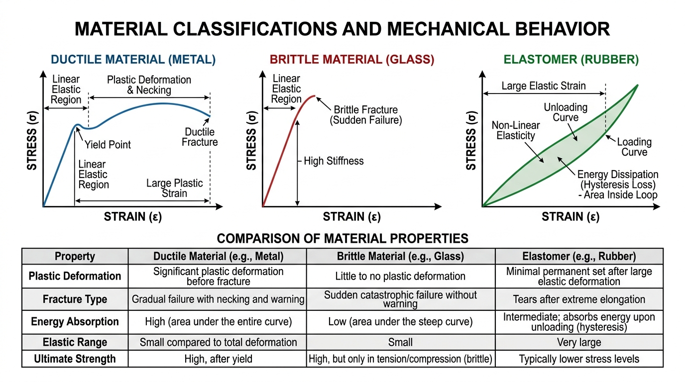
Fig 1.9 — Educational Diagram: Material Classifications (Ductile vs Brittle vs Elastomer Hysteresis)

Overview
Materials respond differently when forces act on them. Mechanical properties describe these responses (deformation, failure) and are quantified by stress, strain and elastic constants. Classifying materials by behaviour helps select the right material for engineering applications.

Basic quantities and definitions

• Stress (σ) = Force/Area = F/A. Unit: Pascal (Pa) = N/m².
• Strain (ε) = Change in length/Original length = ΔL/L. Dimensionless.
• Hooke's law (linear elastic region): σ = E·ε, where E is Young's modulus.
• Elastic limit: maximum stress up to which deformation is fully recoverable. Above it, plastic (permanent) deformation occurs.

Material classifications by mechanical response

• Elastic vs Plastic: Elastic materials return to original shape after load is removed (within elastic limit). Plastic deformation is permanent. Example: rubber (elastic), modeling clay (plastic).
• Ductile vs Brittle: Ductile materials undergo large plastic deformation before fracture (e.g., mild steel); brittle materials fracture with little plastic deformation (e.g., glass, ceramics).
• Malleable vs Non-malleable: Malleability is the ability to deform under compressive stress (sheet forming). Gold is highly malleable; cast iron is not.
• Tough vs Weak: Toughness is the ability to absorb energy before fracture (area under stress–strain curve). Rubber and structural steels are tough; glass is not.
• Hard vs Soft: Hardness resists surface indentation or scratching (diamond = very hard; wax = soft).
• Rigid vs Flexible: Rigidity relates to stiffness (high Young's modulus); flexible materials have low E (rubber, textiles).
• Isotropic vs Anisotropic: Isotropic materials have identical properties in all directions (most metals). Anisotropic (composites, wood) have direction-dependent properties.

Key mechanical properties

• Young's modulus (E) — measure of tensile (or compressive) stiffness: large E → stiffer material.
• Shear modulus (G) — stiffness against shear deformation.
• Bulk modulus (K or B) — resistance to uniform volume change under pressure.
• Poisson's ratio (ν) — lateral contraction per unit longitudinal extension: ν = −ε_lateral/ε_longitudinal.
• Yield strength — stress at which a material begins to deform plastically.
• Ultimate tensile strength (UTS) — maximum stress a material can sustain before necking/fracture.
• Toughness — energy absorbed before fracture (area under stress–strain curve).
• Resilience — energy stored in elastic deformation (area under linear part of curve).

Stress–strain curve (concept)
For a typical ductile metal under tensile testing: proportional limit (linear Hooke's law region) → elastic limit → yield point (plastic flow) → strain hardening → ultimate tensile strength → necking → fracture. For brittle materials the linear region is short and fracture follows soon after the elastic limit.

Relations among elastic constants (for isotropic, linear elastic materials)

• G = E / [2(1 + ν)]
• K = E / [3(1 − 2ν)]

Practical notes
- Engineers select materials balancing stiffness, strength, ductility and toughness according to application (e.g., bridge cables need high tensile strength and ductility; cutting tools need high hardness).
- Temperature, strain rate and microstructure (grain size, defects) significantly affect mechanical behaviour.

Fig 1.10 — Educational Diagram: Bending of Beams, Depression Formula & I-Shaped Girder Design

Scope: In the chapter Mechanical Properties of Solids, units and dimensions help you (a) express physical quantities consistently, (b) check equations by dimensional homogeneity, and (c) guide problem-solving for elasticity (stress, strain, moduli, energy stored).

Units and SI base units:

• Length: metre (m)
• Mass: kilogram (kg)
• Time: second (s)
• Force: newton (N) = kg·m·s⁻²
• Stress / Pressure: pascal (Pa) = N/m² = kg·m⁻¹·s⁻²
• Strain: dimensionless (ratio of lengths)

Dimensions (symbolic): Use [M] for mass, [L] for length, [T] for time. Examples:

• Force F: [M L T⁻²]
• Stress (σ) or Pressure (P): [M L⁻¹ T⁻²]
• Young's modulus Y, Shear modulus G, Bulk modulus K: same dimension as stress
• Strain (ε): dimensionless = [1]

Dimensional analysis & homogeneity:

• Every physically correct equation must be dimensionally homogeneous: both sides must have the same dimensions.
• Use dimensions to check derived expressions and to spot algebraic mistakes (e.g., missing length factor).
• Dimensional analysis cannot give numerical constants (like 1/2) nor choose between dimensionless functions (sin, exp) – it only checks consistency and suggests forms.

Key physical ideas in elasticity:

• Stress = internal force per unit area (normal stress σ = F/A). Unit: Pa.
• Strain = fractional deformation (longitudinal strain ε = ΔL/L). Dimensionless.
• Hooke's law (linear elastic region): stress ∝ strain. The proportionality constant is a modulus (Young's modulus Y for tension/compression).
• Shear stress τ and shear strain γ: τ = G γ, where G is shear modulus.
• Bulk modulus K relates pressure change to fractional volume change: ΔP = −K (ΔV/V).
• Poisson's ratio ν is dimensionless: ν = −(transverse strain)/(longitudinal strain).

Practical problem-solving tips:

1. Read the problem carefully. Identify what is asked, given quantities, geometry and material.
2. List knowns and unknowns with symbols and units. Convert all values to SI units before substituting (e.g., mm → m, cm² → m², kN → N).
3. Write down the governing relation(s) (Hooke's law, σ = F/A, ε = ΔL/L, ΔL = F L/(A Y), τ = F/A, τ = G γ, ΔV/V = −P/K, energy U = 1/2 F ΔL or energy density u = 1/2 σ ε).
4. Check dimensions of the equation. If dimensions don’t match, re-check algebra and units.
5. Use limiting cases to check answers (e.g., if Y → ∞, ΔL → 0; if A increases, ΔL decreases).
6. Sketch the situation and free-body diagrams when needed (show forces, cross-section, deformation ΔL). For composite or series/parallel arrangements, treat segments separately and apply compatibility of strains or equilibrium of forces.
7. Keep track of signs (compression vs tension, volumetric decrease vs applied pressure). Use minus sign for ΔV under positive external pressure when using K definition.
8. Use approximate relations for small angles: tan θ ≈ θ (in radians) when deriving shear strain γ ≈ x/h.
9. Report final answer with appropriate significant figures and units. Always state the physical meaning (e.g., whether deformation is within elastic limit).

These principles make solving elasticity problems systematic, reduce algebraic errors, and ensure physically consistent answers.